『Rによる機械学習』第2版(以降、テキスト)の第6章では回帰法について扱っています。第6.1節で線形回帰、第6.3節でモデル木を解説していますが、実例で使っているデータが異なっており、線形回帰とモデル木の直接的な比較は行われていません。また、第6.4節の実例で利用しているデータの目的変数である品質スコアは間隔尺度というよりは順序尺度的なフィーチャーのようで回帰式を用いて求めるのが適切であるか疑問が残ります。
そこで、本ブログではテキスト第6.2節の線形回帰の実例で使用している医療費データを用いて、線形回帰モデルとモデル木モデルを比較してみます。なお、データやモデルに関する説明はテキストを参照してください。
Packages and Datasets
本ページではR version 3.5.3 (2019-03-11)の標準パッケージ以外に以下の追加パッケージを用いています。
| Package | Version | Description |
|---|---|---|
| Cubist | 0.2.2 | Rule- And Instance-Based Regression Modeling |
| ggplot2 | 3.2.1 | Create Elegant Data Visualisations Using the Grammar of Graphics |
| gridExtra | 2.3 | Miscellaneous Functions for “Grid” Graphics |
| rsample | 0.0.5 | General Resampling Infrastructure |
| tidyverse | 1.2.1 | Easily Install and Load the ‘Tidyverse’ |
また、本ページでは以下のデータセットを用いています。
| Dataset | Package | Version | Description |
|---|---|---|---|
| insurance | NA | NA | dataspelunking/MLwR, GitHub |
対象データ
対象データはシミュレーションにより作成された米国の患者が必要とする仮説的な医療費に関する情報です。テキストに記載されている線形回帰モデルに対する改善策に必要なフィーチャー(age2、bmi30)を追加してあります。
insurance## # A tibble: 1,338 x 9
## age sex bmi children smoker region expenses age2 bmi30
## <int> <fct> <dbl> <int> <fct> <fct> <dbl> <dbl> <dbl>
## 1 19 female 27.9 0 yes southwest 16885. 361 0
## 2 18 male 33.8 1 no southeast 1726. 324 1
## 3 28 male 33 3 no southeast 4449. 784 1
## 4 33 male 22.7 0 no northwest 21984. 1089 0
## 5 32 male 28.9 0 no northwest 3867. 1024 0
## 6 31 female 25.7 0 no southeast 3757. 961 0
## 7 46 female 33.4 1 no southeast 8241. 2116 1
## 8 37 female 27.7 3 no northwest 7282. 1369 0
## 9 37 male 29.8 2 no northeast 6406. 1369 0
## 10 60 female 25.8 0 no northwest 28923. 3600 0
## # ... with 1,328 more rows
線形回帰による予測
テキスト第6章における線形回帰を使った医療費の改良型予測モデルでは、自由度調整済決定係数\(R^2\)値が比較的良好な値を示しています。
insurance %>%
  lm(expenses ~ age + age2 + children + bmi + sex + bmi30*smoker + region,
     data = .) %>%
  summary()
##
## Call:
## lm(formula = expenses ~ age + age2 + children + bmi + sex + bmi30 *
## smoker + region, data = .)
##
## Residuals:
## Min 1Q Median 3Q Max
## -17297.1 -1656.0 -1262.7 -727.8 24161.6
##
## Coefficients:
## Estimate Std. Error t value Pr(>|t|)
## (Intercept) 139.0053 1363.1359 0.102 0.918792
## age -32.6181 59.8250 -0.545 0.585690
## age2 3.7307 0.7463 4.999 6.54e-07 ***
## children 678.6017 105.8855 6.409 2.03e-10 ***
## bmi 119.7715 34.2796 3.494 0.000492 ***
## sexmale -496.7690 244.3713 -2.033 0.042267 *
## bmi30 -997.9355 422.9607 -2.359 0.018449 *
## smokeryes 13404.5952 439.9591 30.468 < 2e-16 ***
## regionnorthwest -279.1661 349.2826 -0.799 0.424285
## regionsoutheast -828.0345 351.6484 -2.355 0.018682 *
## regionsouthwest -1222.1619 350.5314 -3.487 0.000505 ***
## bmi30:smokeryes 19810.1534 604.6769 32.762 < 2e-16 ***
## ---
## Signif. codes: 0 '***' 0.001 '**' 0.01 '*' 0.05 '.' 0.1 ' ' 1
##
## Residual standard error: 4445 on 1326 degrees of freedom
## Multiple R-squared: 0.8664, Adjusted R-squared: 0.8653
## F-statistic: 781.7 on 11 and 1326 DF, p-value: < 2.2e-16このモデルの性能を見るために予測値と観測値の散布図をプロットしてみます。赤点線は「\(予測値 = 観測値\)」となる切片\(0\)、傾き\(1\)の直線で、ドットがこの線に近いほど正しく予測できていると言えます。
gg_ols <- insurance %>%
  lm(expenses ~ age + age2 + children + bmi + sex + bmi30*smoker + region,
     data = .) %>%
  broom::augment() %>%
  ggplot2::ggplot(ggplot2::aes(x = expenses, y = .fitted)) +
    ggplot2::geom_abline(slope = 1, colour = "red", linetype = "dotted") +
    ggplot2::geom_point() +
    ggplot2::labs(title = "予測値-観測値プロット(線形回帰)",
                  x = "観測値", y = "予測値")
gg_ols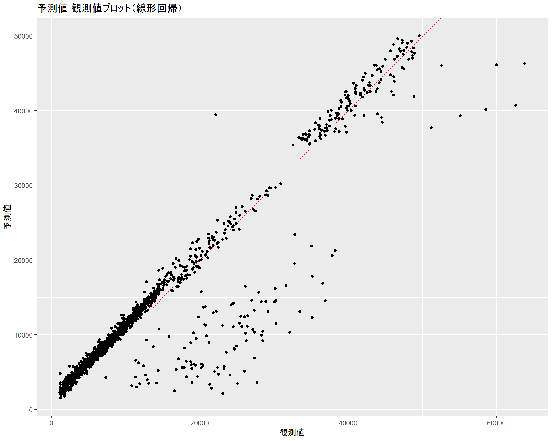
残差の分布傾向も合わせて確認しておきます。赤点線は\(残差 = 0\)となる直線です。
gg_ols_resid <- insurance %>%
  lm(expenses ~ age + age2 + children + bmi + sex + bmi30*smoker + region,
     data = .) %>%
  broom::augment() %>%
  ggplot2::ggplot(ggplot2::aes(x = .fitted, y = .resid)) +
    ggplot2::geom_hline(yintercept = 0, colour = "red", linetype = "dotted") +
    ggplot2::geom_point() + ggplot2::ylim(-20000, 30000) +
    ggplot2::labs(title = "残差プロット(線形回帰)", x = "予測値", y = "残差")
gg_ols_resid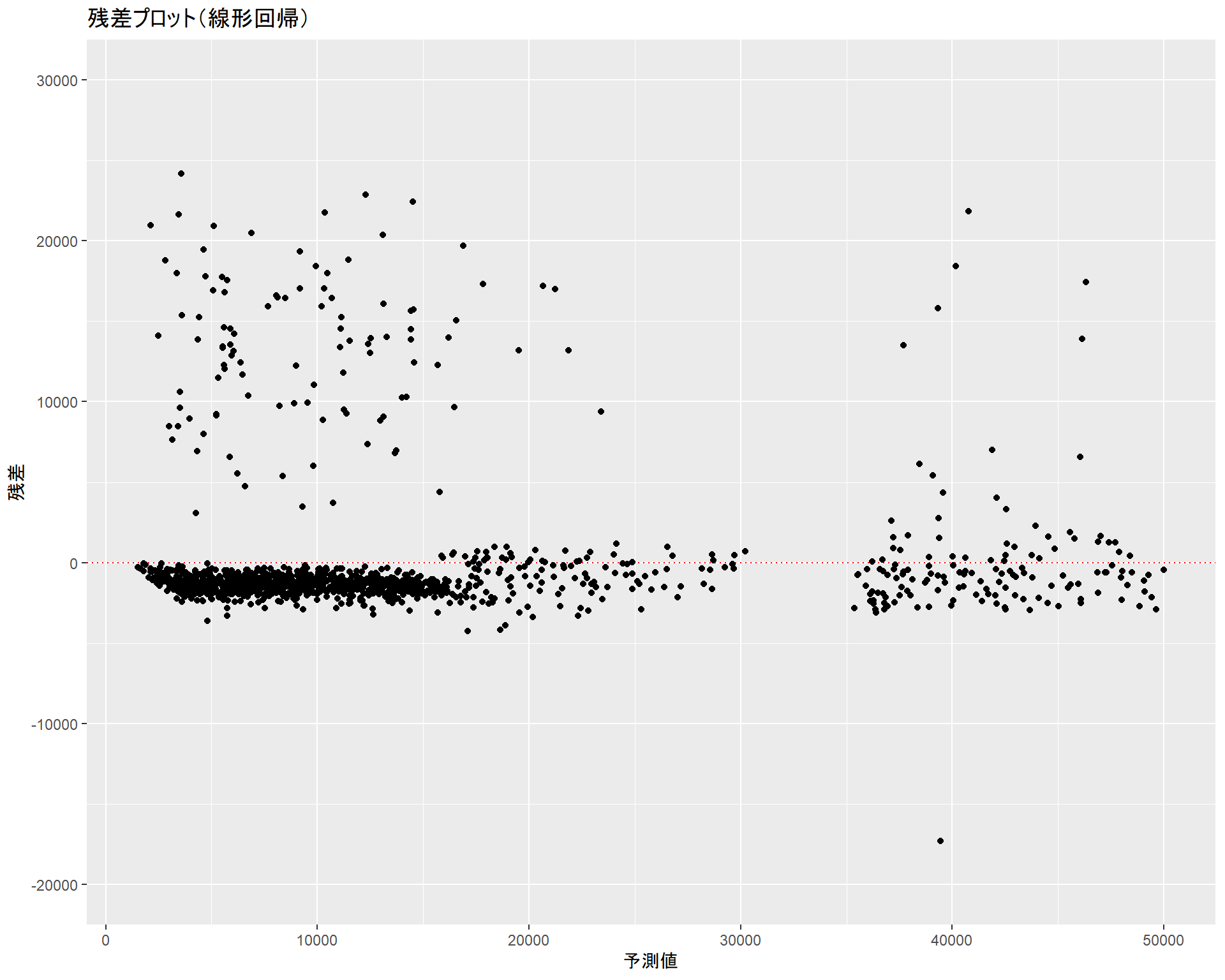
モデル木による予測
第6.4節で扱ったモデル木(ルール・インスタンスベース)を適用してみます。ここでは、RWekaパッケージではなくCubistパッケージを用いています。
データの分割
最初にinsuranceデータフレームをトレーニング用とテスト用に分割します。線形回帰用に追加した非線形項(age2とbmi30)は外しておきます。なお、分割比率はデフォルトの\(3:1\)です。
ins_train## # A tibble: 1,004 x 7
## age sex bmi children smoker region expenses
## <int> <fct> <dbl> <int> <fct> <fct> <dbl>
## 1 19 female 27.9 0 yes southwest 16885.
## 2 18 male 33.8 1 no southeast 1726.
## 3 28 male 33 3 no southeast 4449.
## 4 32 male 28.9 0 no northwest 3867.
## 5 46 female 33.4 1 no southeast 8241.
## 6 37 female 27.7 3 no northwest 7282.
## 7 37 male 29.8 2 no northeast 6406.
## 8 60 female 25.8 0 no northwest 28923.
## 9 62 female 26.3 0 yes southeast 27809.
## 10 23 male 34.4 0 no southwest 1827.
## # ... with 994 more rowsins_test## # A tibble: 334 x 7
## age sex bmi children smoker region expenses
## <int> <fct> <dbl> <int> <fct> <fct> <dbl>
## 1 33 male 22.7 0 no northwest 21984.
## 2 31 female 25.7 0 no southeast 3757.
## 3 25 male 26.2 0 no northeast 2721.
## 4 19 male 24.6 1 no southwest 1837.
## 5 52 female 30.8 1 no northeast 10797.
## 6 18 male 34.1 0 no southeast 1137.
## 7 55 female 32.8 2 no northwest 12269.
## 8 63 male 28.3 0 no northwest 13770.
## 9 19 male 20.4 0 no northwest 1625.
## 10 26 male 20.8 0 no southwest 2302.
## # ... with 324 more rows
モデルの作成
トレーニング用データを用いてモデルを作成します。
m_ins <- Cubist::cubist(ins_train[, -7], ins_train[, 7])
m_ins
##
## Call:
## cubist.default(x = ins_train[, -7], y = ins_train[, 7])
##
## Number of samples: 1004
## Number of predictors: 6
##
## Number of committees: 1
## Number of rules: 4モデルのルールは以下の通りです。
m_ins %>%
  summary()
##
## Call:
## cubist.default(x = ins_train[, -7], y = ins_train[, 7])
##
##
## Cubist [Release 2.07 GPL Edition] Wed Nov 20 13:03:03 2019
## ---------------------------------
##
## Target attribute `outcome'
##
## Read 1004 cases (7 attributes) from undefined.data
##
## Model:
##
## Rule 1: [253 cases, mean 4366.201, range 1135.94 to 27724.29, est err 2023.477]
##
## if
## age <= 29
## smoker = no
## then
## outcome = -2678.36 + 214 age + 820 children
##
## Rule 2: [549 cases, mean 10118.000, range 3260.2 to 36910.61, est err 1510.557]
##
## if
## age > 29
## smoker = no
## then
## outcome = -6384.48 + 315 age + 506 children
##
## Rule 3: [97 cases, mean 21791.002, range 12829.46 to 38245.59, est err 1991.133]
##
## if
## bmi <= 30.1
## smoker = yes
## then
## outcome = 1722.86 + 247 age + 374 bmi + 125 children
##
## Rule 4: [105 cases, mean 41641.012, range 32548.34 to 62592.87, est err 1462.996]
##
## if
## bmi > 30.1
## smoker = yes
## then
## outcome = 14924.378 + 271 age + 425 bmi + 210 children
##
##
## Evaluation on training data (1004 cases):
##
## Average |error| 2570.024
## Relative |error| 0.28
## Correlation coefficient 0.88
##
##
## Attribute usage:
## Conds Model
##
## 100% smoker
## 80% 100% age
## 20% 20% bmi
## 100% children
##
##
## Time: 0.0 secs
結果の読み方
Cubist::cubist関数の出力の読み方を簡単に説明しておきます。以下の出力例と上の出力の内容が異なっている場合がありますが、その場合は気にしないでください。
Model:

  Rule 1: [253 cases, mean 4366.201, range 1135.94 to 27724.29, est err 2023.477]

    if
    age <= 29
    smoker = no
    then
outcome = -2678.36 + 214 age + 820 children Model項はモデル木のルールが表示されています。
| item | description |
|---|---|
| Rule | ルール番号とルールに該当するインスタンス数、その平均値、その範囲、推定誤差 |
| if | 分類ルール(分類条件・ケース) |
| then | 分類ルールを満たす場合の回帰式(\(y = \beta_0 + \beta_1x_1 + \beta_2 x_2 \ldots\)) |
Evaluation on training data (1004 cases):

    Average  |error|           2570.024
    Relative |error|               0.28
Correlation coefficient 0.88 Evaluation項は学習モデルの評価結果です。
| item | description |
|---|---|
| Average |error| | 平均絶対誤差(MAE) |
| Relative |error| | 相対絶対誤差(RAE)、\(1\)未満ならば有用なモデルと見なせる |
| Correlation coefficient | 観測値と予測値の相関係数(\(R\)) |
    Attribute usage:
      Conds  Model

      100%           smoker
       80%   100%    age
       20%    20%    bmi
             100%    children
Attribute usage項は、分類ルール(Conds)や回帰式(Model)で使われているインスタンス数の割合をフィーチャーごとに表したものです。
| item | description |
|---|---|
| Conds | 分類ルール(分類条件・ケース)で使われているフィーチャーごとのインスタンス数の割合(\(1\%\)未満の場合は非表示) |
| Model | 回帰式に使われているフィーチャーごとのインスタンス数の割合(\(1\%\)未満の場合は非表示) |
この例では、ageというフィーチャーは分類ルール\(1\)と\(2\)で使われており、分類ルール\(1\)と\(2\)にはそれぞれ\(253\)と\(549\)のインスタンスがありましたので、\(\frac{253 + 549}{1004} = 80\%\)となっています。
bmiというフィーチャーは分類ルール\(3\)と\(4\)の回帰式で使われており、分類ルール\(3\)と\(4\)にはそれぞれ\(97\)と\(105\)のインスタンスがありましたので、\(\frac{95 + 105}{1004} = 20\%\)となっています。
モデルを用いた予測
作成したモデルにテスト用データを適用してモデル精度を確認します。線形回帰モデルと比較するために線形回帰モデルのときと同じプロットを行います。
p_ins <- m_ins %>%
  predict(ins_test)

ins_test %>%
  dplyr::bind_cols(pred = p_ins) %>%
  ggplot2::ggplot(ggplot2::aes(x = expenses, y = pred)) +
    ggplot2::geom_abline(slope = 1, colour = "red", linetype = "dotted") +
    ggplot2::geom_point() +
    ggplot2::labs(title = "予測値-観測値プロット(モデル木)",
                  x = "観測値", y = "予測値")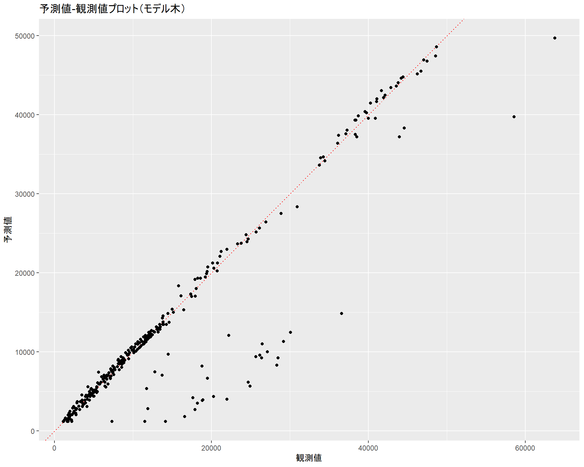
ins_test %>%
  dplyr::bind_cols(pred = p_ins) %>%
  dplyr::mutate(resid = expenses - pred) %>%
  ggplot2::ggplot(ggplot2::aes(x = pred, y = resid)) +
    ggplot2::geom_hline(yintercept = 0, colour = "red", linetype = "dotted") +
    ggplot2::geom_point() + ggplot2::ylim(-20000, 30000) +
    ggplot2::labs(title = "残差プロット(モデル木)", x = "予測値", y = "残差")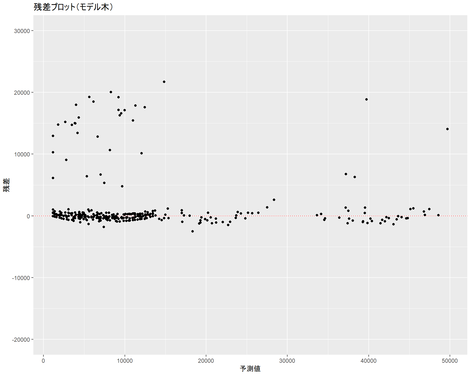
ins_test %>%
  dplyr::bind_cols(pred = p_ins) %>%
  with(cor(expenses, pred))
## [1] 0.9296292相関係数もかなり高く、まずまずのモデルになっていると言えます。
全データに対する予測
線形回帰モデルと比較を行うために全データに対する予測を行います。こちらでも線形回帰用に追加した非線形項(age2とbmi30)を外します。
p_ins <- insurance %>%
  dplyr::select(-age2, -bmi30) %>%
  predict(m_ins, .)

gg_cubist <- insurance %>%
  dplyr::select(-age2, -bmi30) %>%
  dplyr::bind_cols(pred = p_ins) %>%
  ggplot2::ggplot(ggplot2::aes(x = expenses, y = pred)) +
    ggplot2::geom_abline(slope = 1, colour = "red", linetype = "dotted") +
    ggplot2::geom_point() +
    ggplot2::labs(title = "予測値-観測値プロット(モデル木)",
                  x = "観測値", y = "予測値")
gg_cubist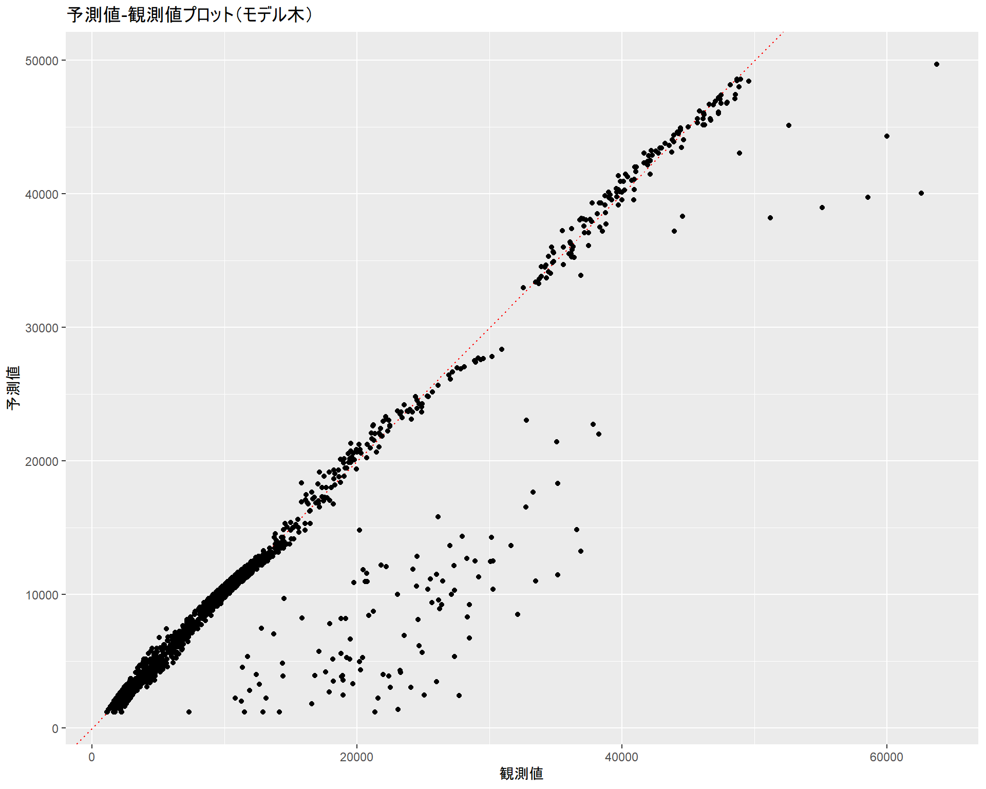
gg_cubist_resid <- insurance %>%
  dplyr::select(-age2, -bmi30) %>%
  dplyr::bind_cols(pred = p_ins) %>%
  dplyr::mutate(resid = expenses - pred) %>%
  ggplot2::ggplot(ggplot2::aes(x = pred, y = resid)) +
    ggplot2::geom_hline(yintercept = 0, colour = "red", linetype = "dotted") +
    ggplot2::geom_point() + ggplot2::ylim(-20000, 30000) +
    ggplot2::labs(title = "残差プロット(モデル木)", x = "予測値", y = "残差")
gg_cubist_resid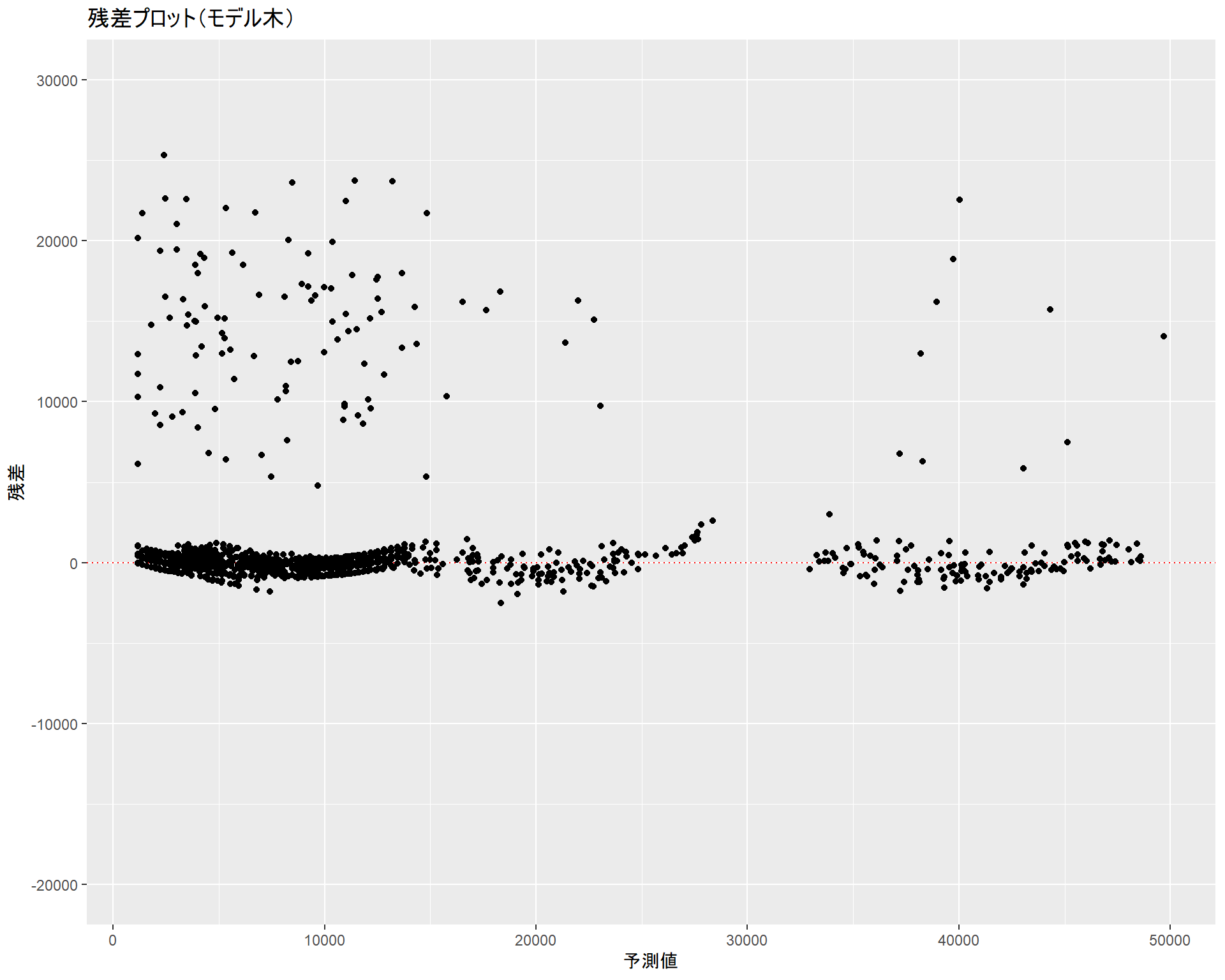
結果比較
線形回帰、モデル木ともに予測から外れるインスタンスの傾向は似ています。しかし、モデル木では線形回帰で使用した非線形項(age2、bmi30)を外しているにもかかわらず線形回帰と同等と言える分布であり、より単純なデータで同等の予測が行えていることが分かります。加えて、ドットの散らばり具合を見る限りではモデル木の方が予測精度が良いと言えます。
gridExtra::grid.arrange(gg_ols, gg_cubist, gg_ols_resid, gg_cubist_resid, ncol = 2)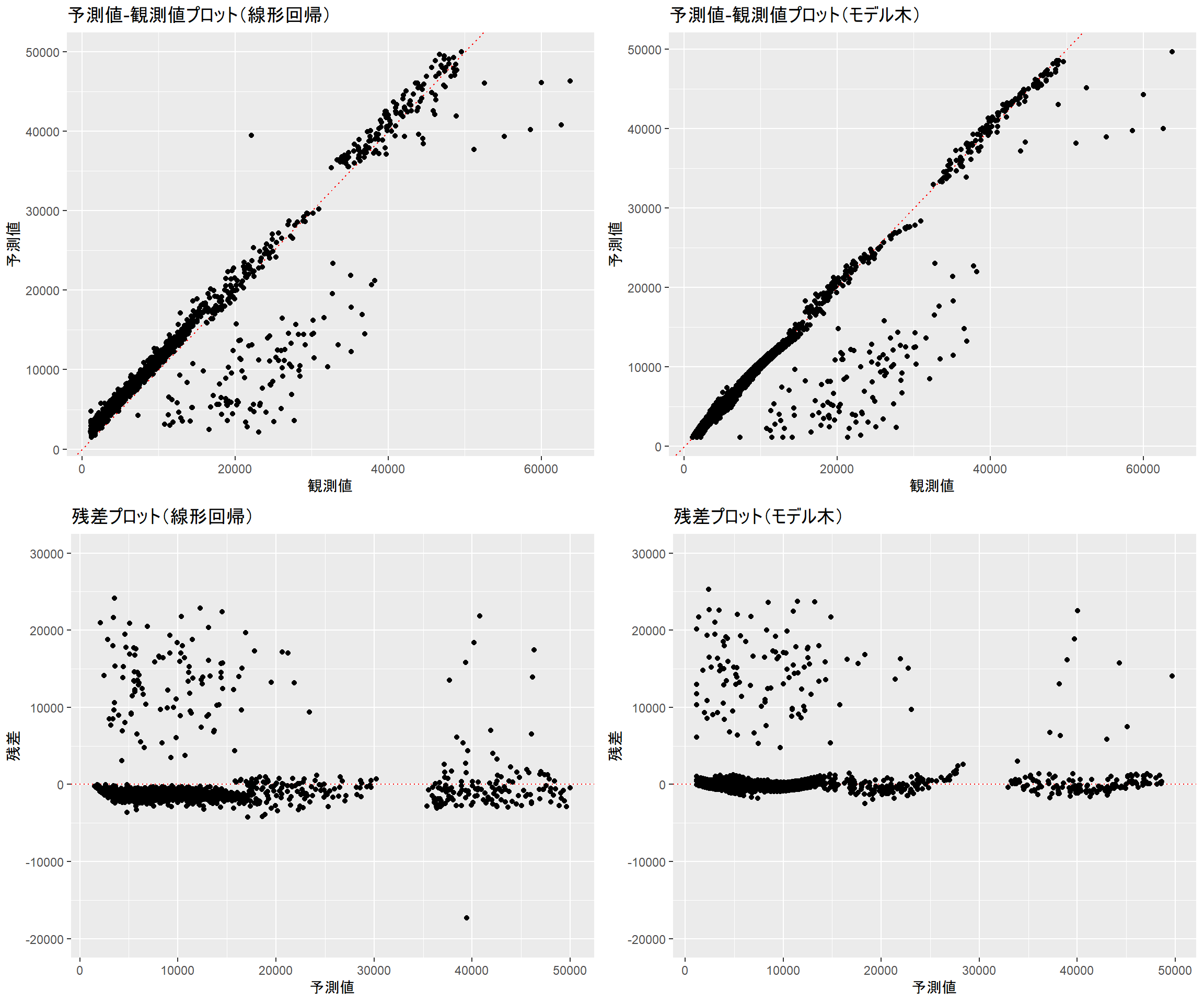
まとめ
テキストでは主観的な目的変数(品質スコア)をモデリングするためにモデル木や回帰木を用いていましたが、本ブログではそれとは異なる目的変数(医療費)をモデリングするためにモデル木を用いてみました。
今回の対象データに対してモデル木は線形回帰モデルよりも予測性能が高い(と思われる)モデルを作成することができました。線形回帰モデルで苦戦している場合は、モデル木モデルを作成して比較してみるのも手だと思います。
Enjoy!