決定木(二分木)の描画にはrpart.plotパッケージが便利です。これらのパッケージでは関数のオプションパラメータの指定により様々な表現ができます。
Packages and Datasets
本ページではR version 3.6.1 (2019-07-05)の標準パッケージ以外に以下の追加パッケージを用いています。
| Package | Version | Description |
|---|---|---|
| knitr | 1.24 | A General-Purpose Package for Dynamic Report Generation in R |
| rpart | 4.1.15 | Recursive Partitioning and Regression Trees |
| rpart.plot | 3.0.8 | Plot ‘rpart’ Models: An Enhanced Version of ‘plot.rpart’ |
| tidyverse | 1.2.1 | Easily Install and Load the ‘Tidyverse’ |
また、本ページでは以下のデータセットを用いています。
| Dataset | Package | Version | Description |
|---|---|---|---|
| TitanicSurvival | carData | 3.0.2 | Survival of passengers on the Titanic |
決定木を作成する
可視化対象となるTitanicSurvivalデータセットは以下のようなデータです。
carData::TitanicSurvival| survived | sex | age | passengerClass | |
|---|---|---|---|---|
| Allen, Miss. Elisabeth Walton | yes | female | 29 | 1st |
| Allison, Master. Hudson Trevor | yes | male | 0.92 | 1st |
| Allison, Miss. Helen Loraine | no | female | 2 | 1st |
| … | NA | NA | … | NA |
| Zakarian, Mr. Mapriededer | no | male | 26.5 | 3rd |
| Zakarian, Mr. Ortin | no | male | 27 | 3rd |
| Zimmerman, Mr. Leo | no | male | 29 | 3rd |
生存者(survived)の人数と比率は以下のようになっています。
carData::TitanicSurvival$survived %>%
  table() %>% print() %>%
prop.table()## .
## no yes
## 809 500## .
## no yes
## 0.618029 0.381971
survivedをキーに決定木を作成します。
dt <- carData::TitanicSurvival %>%
  rpart::rpart(survived ~ ., data = .)

dt## n= 1309
##
## node), split, n, loss, yval, (yprob)
## * denotes terminal node
##
## 1) root 1309 500 no (0.6180290 0.3819710)
## 2) sex=male 843 161 no (0.8090154 0.1909846)
## 4) age>=9.5 800 136 no (0.8300000 0.1700000) *
## 5) age< 9.5 43 18 yes (0.4186047 0.5813953)
## 10) passengerClass=3rd 29 11 no (0.6206897 0.3793103) *
## 11) passengerClass=1st,2nd 14 0 yes (0.0000000 1.0000000) *
## 3) sex=female 466 127 yes (0.2725322 0.7274678) *
決定木を可視化する
作成した決定木をrpart.plot関数を用いて可視化してみます。
dt %>%
  rpart.plot::rpart.plot()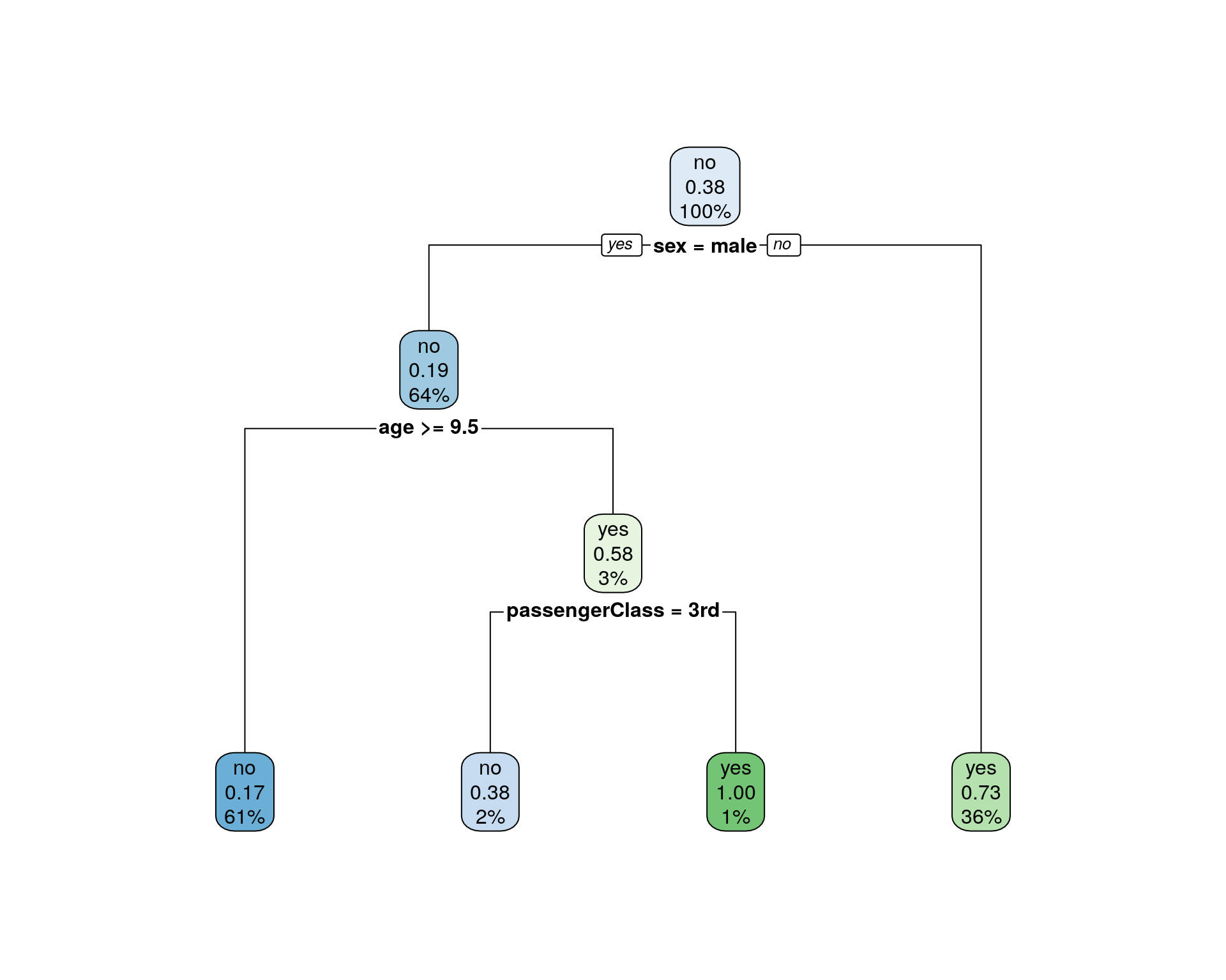
決定木プロットの読み方は以下のようになります。
- ノード(枠の中)の表示は上から順に
survivedのデータで比率の高い方の水準を表示- 生存者(
survived == yes)の比率 - 全データ数に占める割合
- エレメント(枠の下)の数式は決定木の分割条件式
- 分割条件式を満たす場合(判定が
TRUE)は左側へ - 分割条件式を満たせない場合(判定が
FALSE)は右側へ
- 分割条件式を満たす場合(判定が
- ノードの色が濃いほどエントロピーが低い
ですので、最初の分割は性別(sex)が男(mail)か否かで分類され
- 左側(性別が男)
- 死亡者の方が多く、内、生存者は0.19、全体の64%
- 右側(性別が女)
- 生存者の方が多く、内、生存者は0.73、全体の36%
となっています。その通りか確認してみます。
左側の場合(sex = mail is yes)
carData::TitanicSurvival %>%
  dplyr::filter(sex == "male") %>%
  .$survived %>%
table() %>% prop.table()## .
## no yes
## 0.8090154 0.1909846
右側の場合(sex = mail is no)
carData::TitanicSurvival %>%
  dplyr::filter(sex != "male") %>%
  .$survived %>%
table() %>% prop.table()## .
## no yes
## 0.2725322 0.7274678
オプションを指定する
デフォルトの表示では直感的に分かりにくい印象があるのでオプションを指定して表示を変更してみます。 表示に関連するオプションは以下の通りです。
| option | values | default | description |
|---|---|---|---|
| type | 0, 1, 2, 3, 4, 5 | 2 | Type of plot |
| extra | 0, 1, 2, 3, 4, 5, 6, 7, 8, 9, +100, auto | auto | Display extra information at the nodes |
typeオプション
| type | description |
|---|---|
| 0 | Draw a split label at each split and a node label at each leaf. |
| 1 | Label all nodes, not just leaves. Similar to text.rpart’s all=TRUE. |
| 2 | Default. Like 1 but draw the split labels below the node labels. Similar to the plots in the CART book. |
| 3 | Draw separate split labels for the left and right directions. |
| 4 | Like 3 but label all nodes, not just leaves. Similar to text.rpart’s fancy=TRUE. See also clip.right.labs. |
| 5 | New in version 2.2.0. Show the split variable name in the interior nodes. |
type = 0
Draw a split label at each split and a node label at each leaf.
dt %>%
  rpart.plot::rpart.plot(type = 0, main = "type = 0")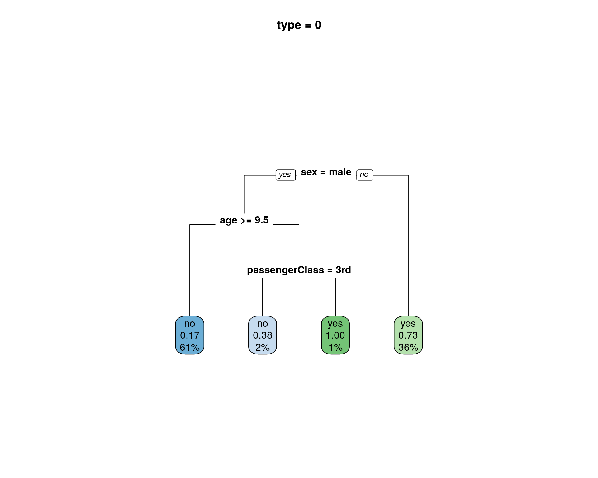
type = 1
Label all nodes, not just leaves. Similar to text.rpart’s all=TRUE.
dt %>%
  rpart.plot::rpart.plot(type = 1, main = "type = 1")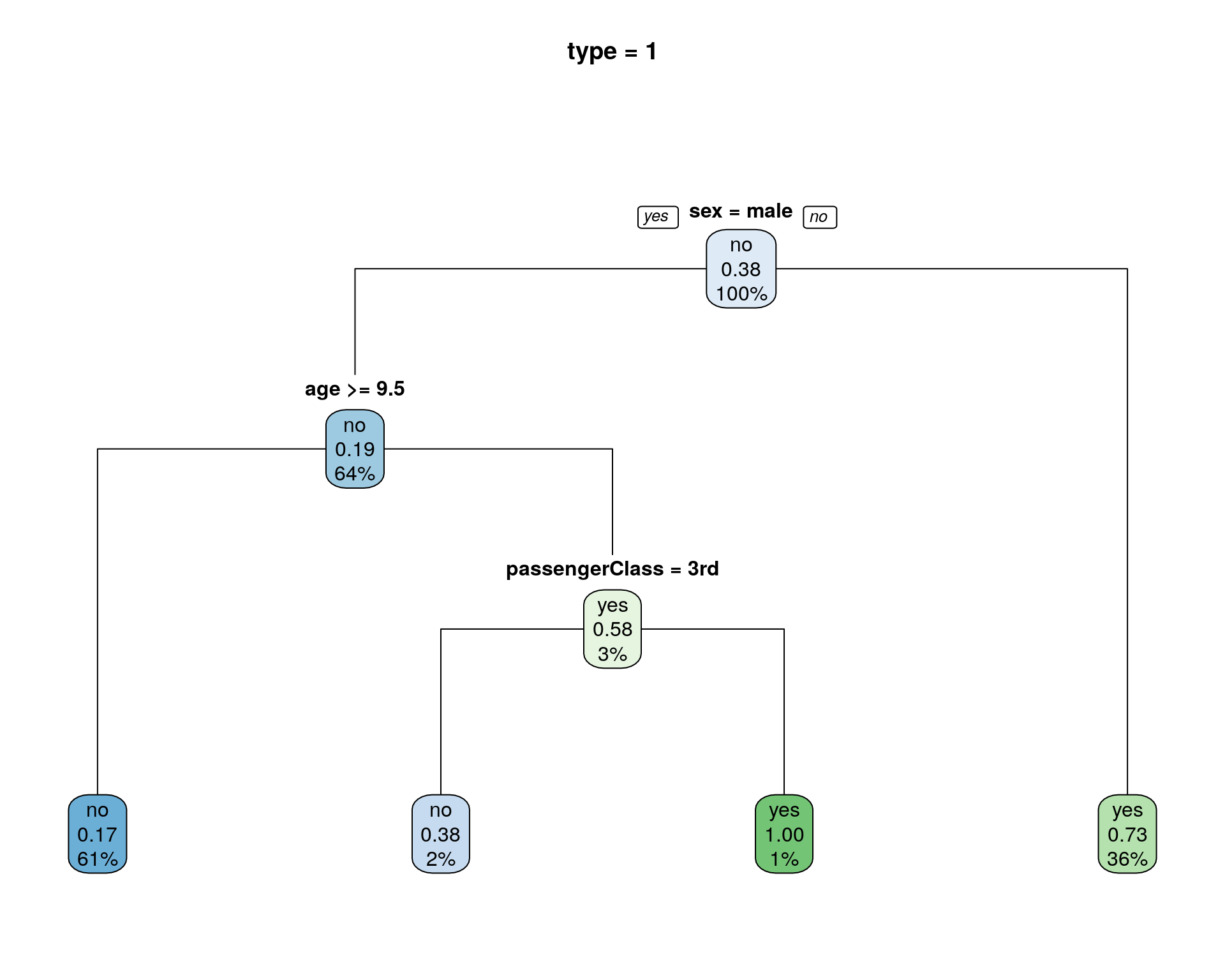
type = 2
Like 1 but draw the split labels below the node labels. Similar to the plots in the CART book.
dt %>%
  rpart.plot::rpart.plot(type = 2, main = "type = 2, as default")
type = 3
Draw separate split labels for the left and right directions.
dt %>%
  rpart.plot::rpart.plot(type = 3, main = "type = 3")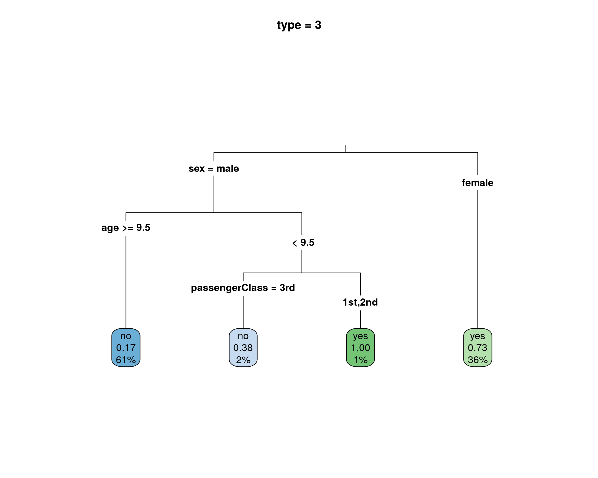
type = 4
Like 3 but label all nodes, not just leaves. Similar to text.rpart’s fancy=TRUE. See also clip.right.labs.
dt %>%
  rpart.plot::rpart.plot(type = 4, main = "type = 4")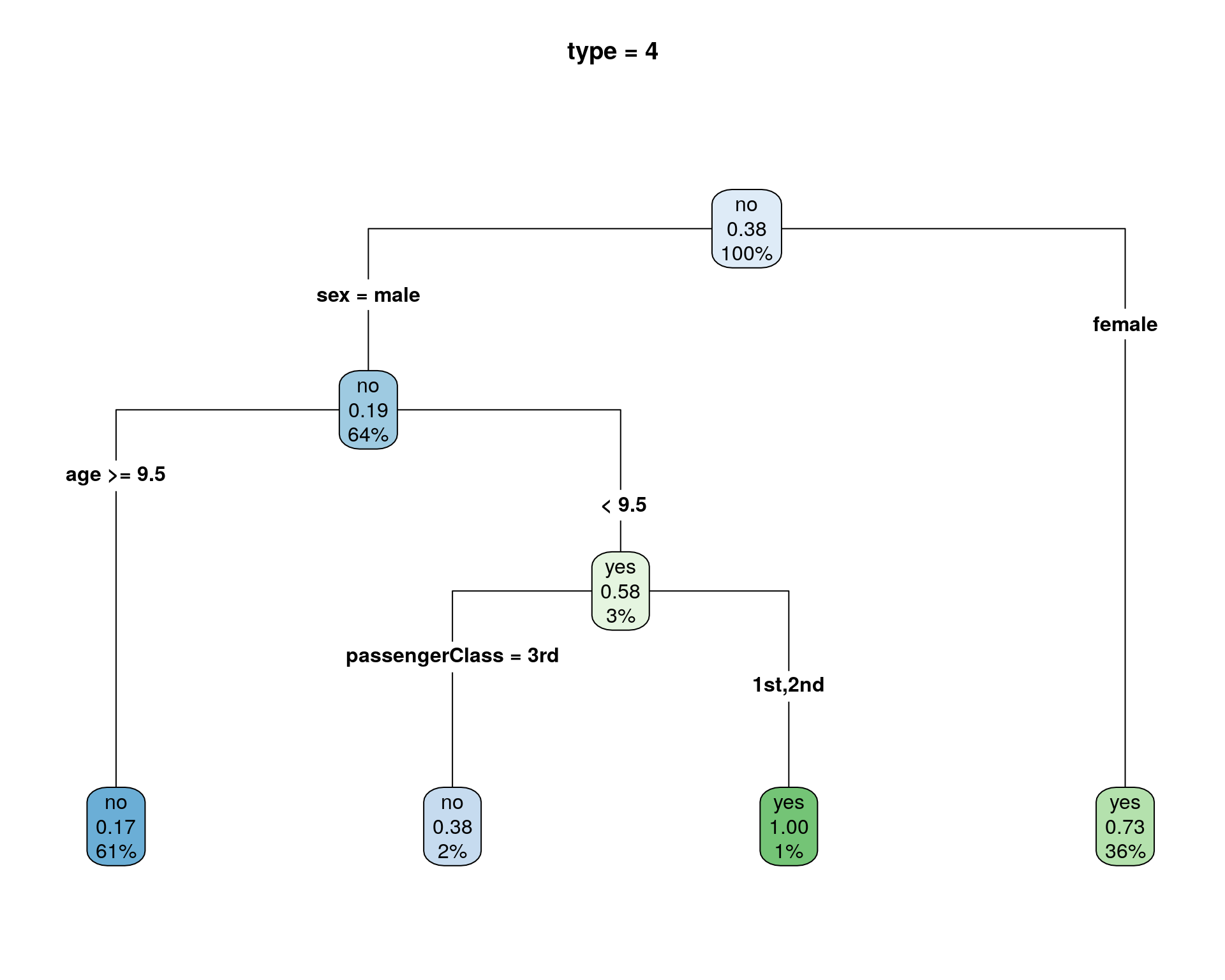
type = 5
New in version 2.2.0. Show the split variable name in the interior nodes.
dt %>%
  rpart.plot::rpart.plot(type = 5, main = "type = 5")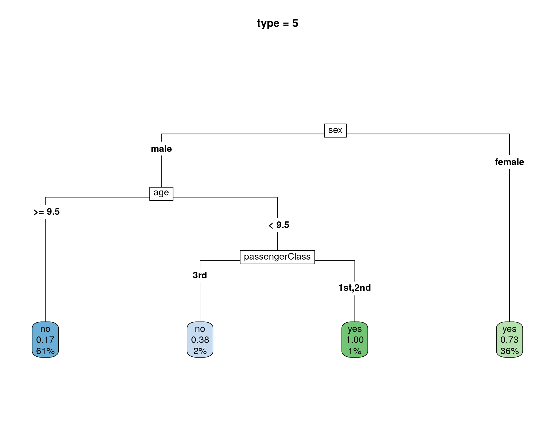
extraオプション
extraオプションは、typeオプションと異なりデフォルトはauto(自動選択)になっています。自動選択は以下の組み合わせからの選択となります。
| extra | description |
|---|---|
| 106 | class model with a binary response(二分木の場合) |
| 104 | class model with a response having more than two levels(三分木以上の場合) |
| 100 | other models(その他の場合) |
auto以外の指定は以下の通りです。
| extra | description |
|---|---|
| 0 | No extra information. |
| 1 | Display the number of observations that fall in the node (per class for class objects; prefixed by the number of events for poisson and exp models). Similar to text.rpart’s use.n=TRUE. |
| 2 | Class models: display the classification rate at the node, expressed as the number of correct classifications and the number of observations in the node. |
| 3 | Class models: misclassification rate at the node, expressed as the number of incorrect classifications and the number of observations in the node. |
| 4 | Class models: probability per class of observations in the node (conditioned on the node, sum across a node is 1). |
| 5 | Class models: like 4 but don’t display the fitted class. |
| 6 | Class models: the probability of the second class only. Useful for binary responses. |
| 7 | Class models: like 6 but don’t display the fitted class. |
| 8 | Class models: the probability of the fitted class. |
| 9 | Class models: The probability relative to all observations – the sum of these probabilities across all leaves is 1. This is in contrast to the options above, which give the probability relative to observations falling in the node – the sum of the probabilities across the node is 1. |
| 10 | New in version 2.2.0. Class models: Like 9 but display the probability of the second class only. Useful for binary responses. |
| 11 | New in version 2.2.0. Class models: Like 10 but don’t display the fitted class. |
| +100 | Add 100 to any of the above to also display the percentage of observations in the node. For example extra=101 displays the number and percentage of observations in the node. Actually, it’s a weighted percentage using the weights passed to rpart. |
extra = "auto"
dt %>%
  rpart.plot::rpart.plot(extra = "auto", main = 'extra = "auto"')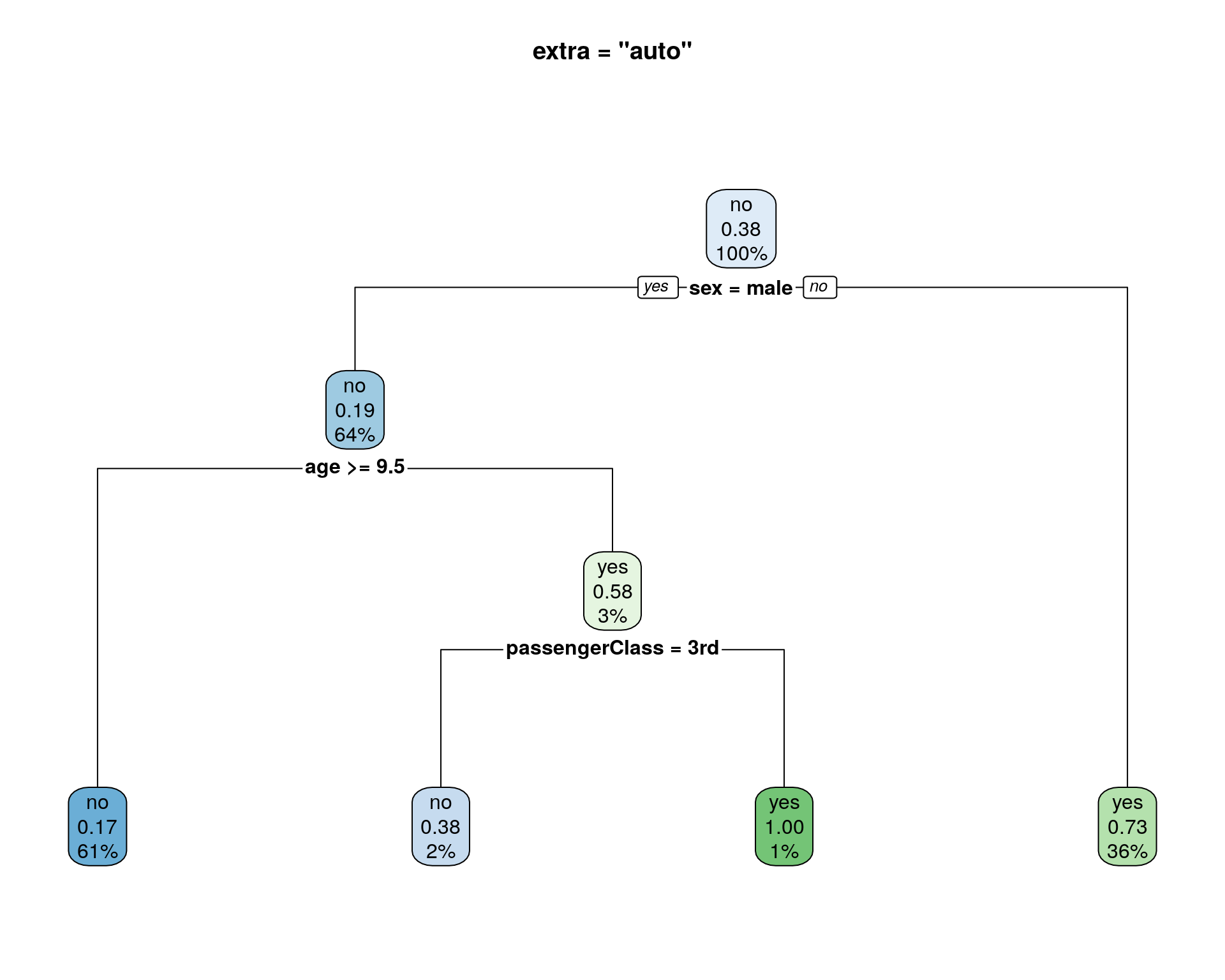
extra = 0
No extra information.
dt %>%
  rpart.plot::rpart.plot(extra = 0, main = "extra = 0")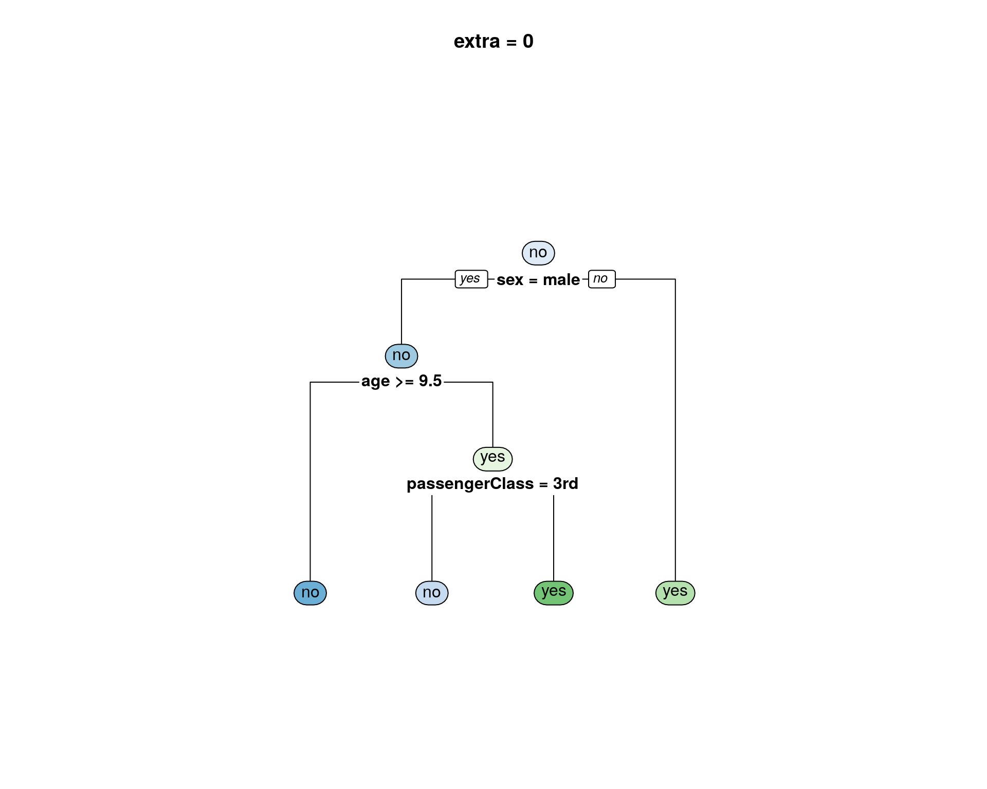
extra = 1
Display the number of observations that fall in the node (per class for class objects; prefixed by the number of events for poisson and exp models). Similar to text.rpart’s use.n=TRUE.
dt %>%
  rpart.plot::rpart.plot(extra = 1, main = "extra = 1")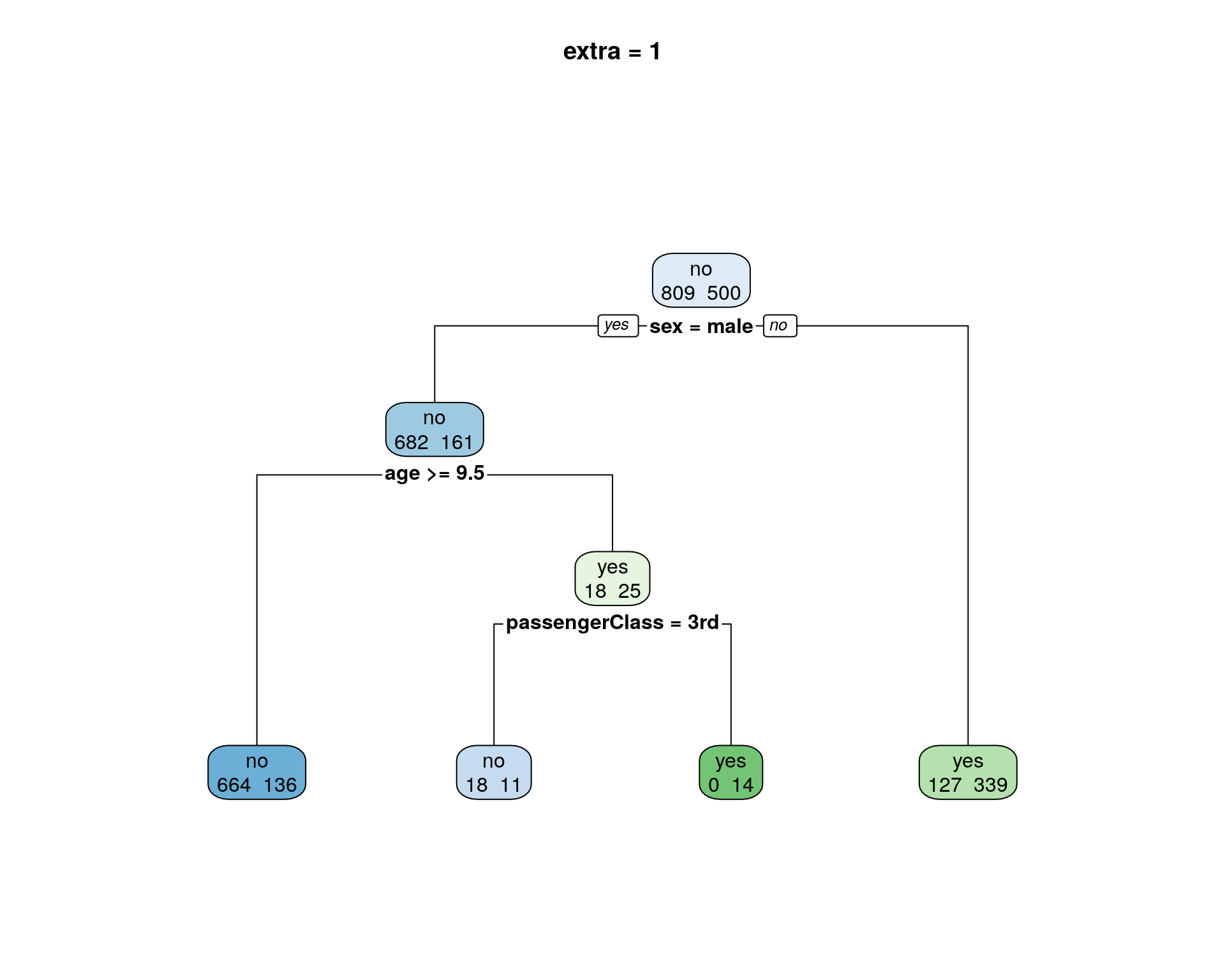
extra = 2
Class models: display the classification rate at the node, expressed as the number of correct classifications and the number of observations in the node.
dt %>%
  rpart.plot::rpart.plot(extra = 2, main = "extra = 2")
extra = 3
Class models: misclassification rate at the node, expressed as the number of incorrect classifications and the number of observations in the node.
dt %>%
  rpart.plot::rpart.plot(extra = 3, main = "extra = 3")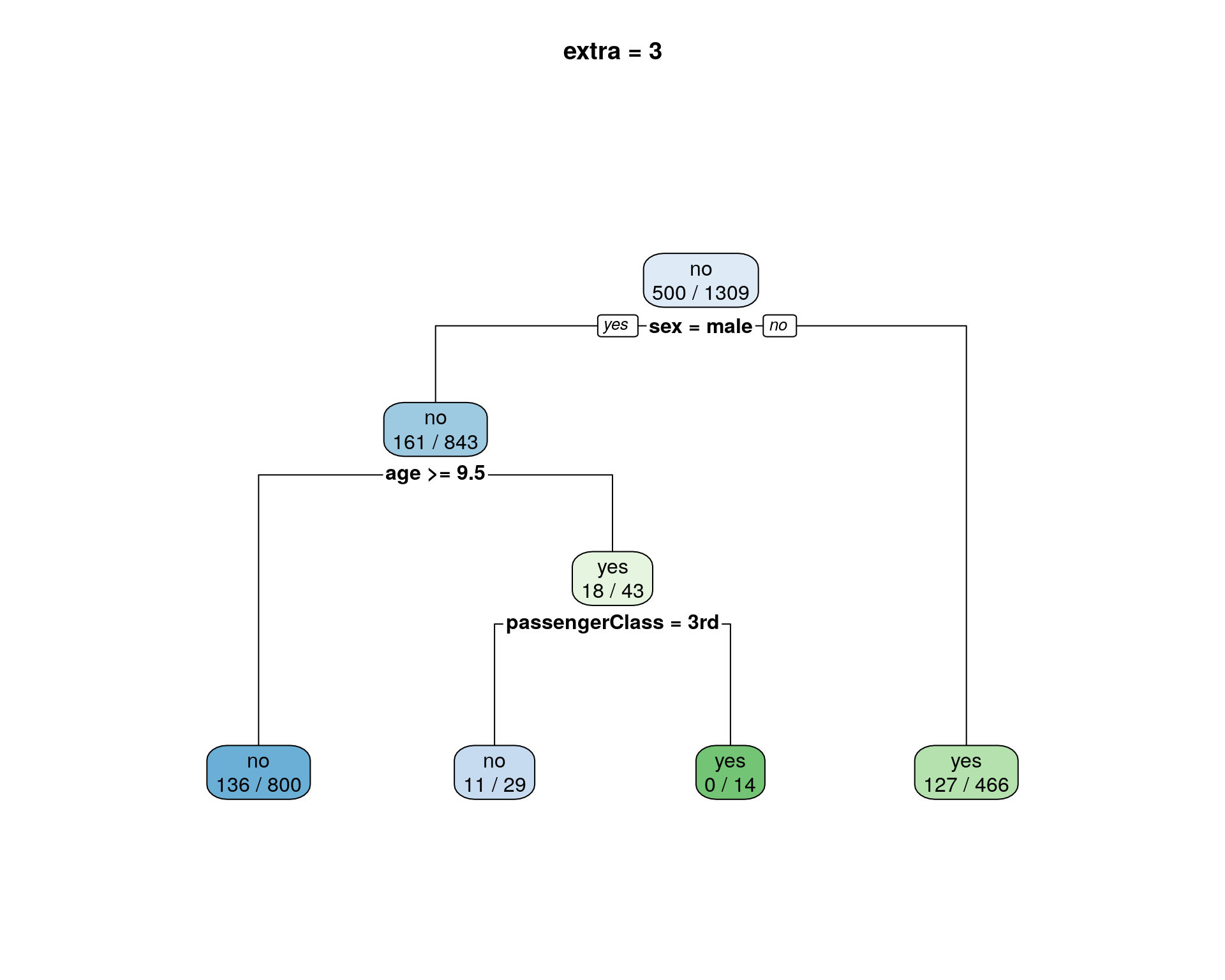
extra = 4
Class models: probability per class of observations in the node (conditioned on the node, sum across a node is 1).
dt %>%
  rpart.plot::rpart.plot(extra = 4, main = "extra = 4")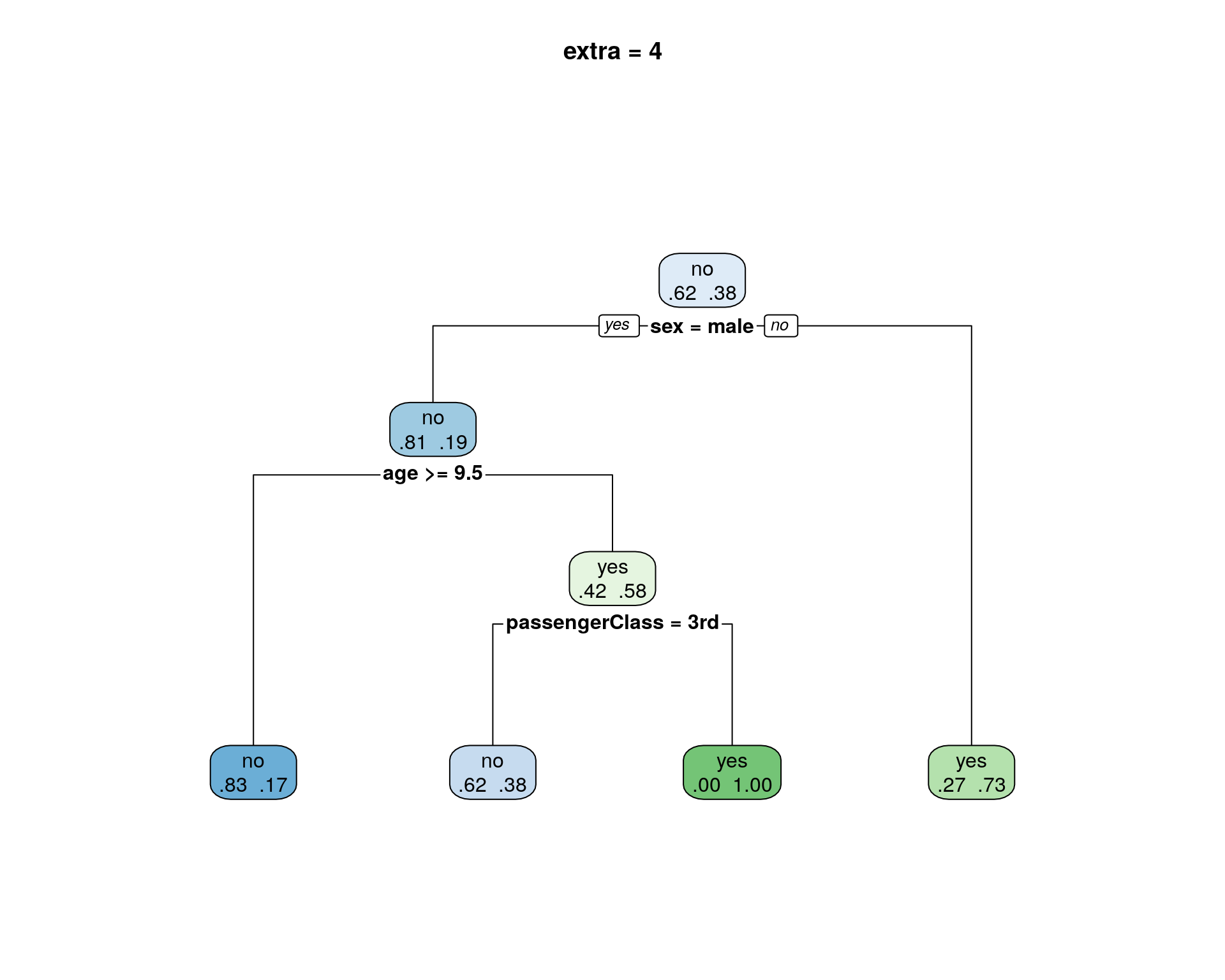
extra = 5
Class models: like 4 but don’t display the fitted class.
dt %>%
  rpart.plot::rpart.plot(extra = 5, main = "extra = 5")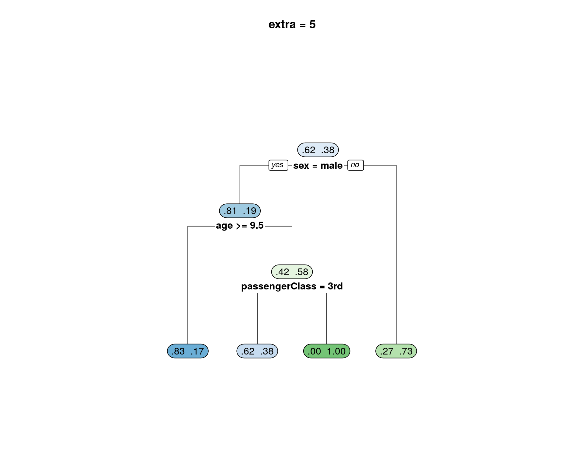
extra = 6
Class models: the probability of the second class only. Useful for binary responses.
dt %>%
  rpart.plot::rpart.plot(extra = 6, main = "extra = 6")
extra = 7
Class models: like 6 but don’t display the fitted class.
dt %>%
  rpart.plot::rpart.plot(extra = 7, main = "extra = 7")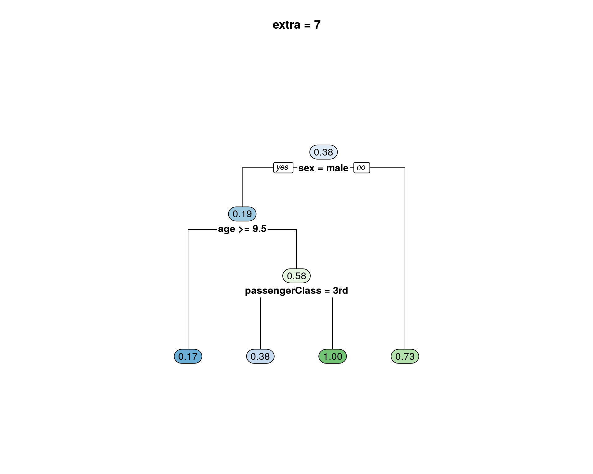
extra = 8
Class models: the probability of the fitted class.
dt %>%
  rpart.plot::rpart.plot(extra = 8, main = "extra = 8")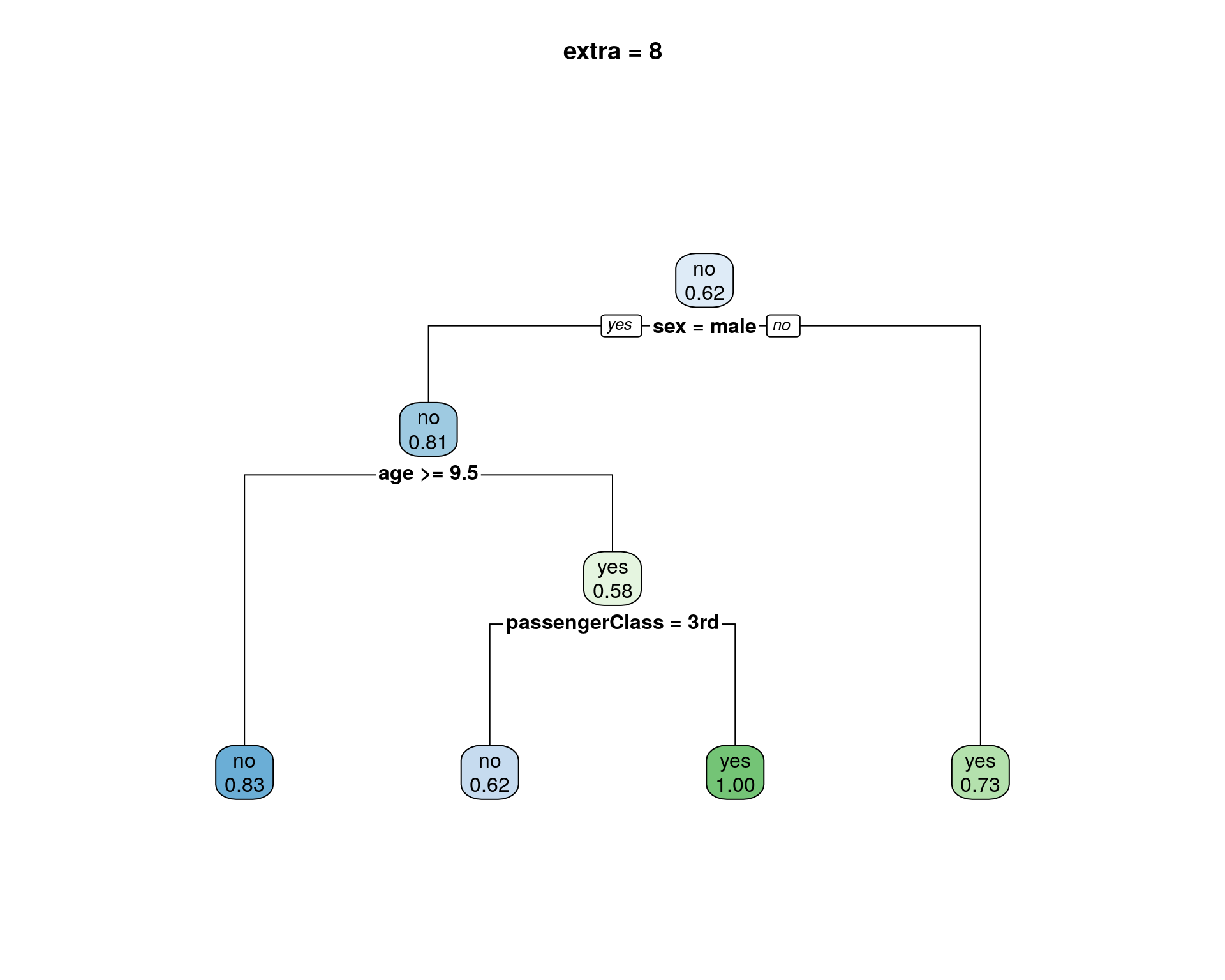
extra = 9
Class models: The probability relative to all observations – the sum of these probabilities across all leaves is 1. This is in contrast to the options above, which give the probability relative to observations falling in the node – the sum of the probabilities across the node is 1.
dt %>%
  rpart.plot::rpart.plot(extra = 9, main = "extra = 9")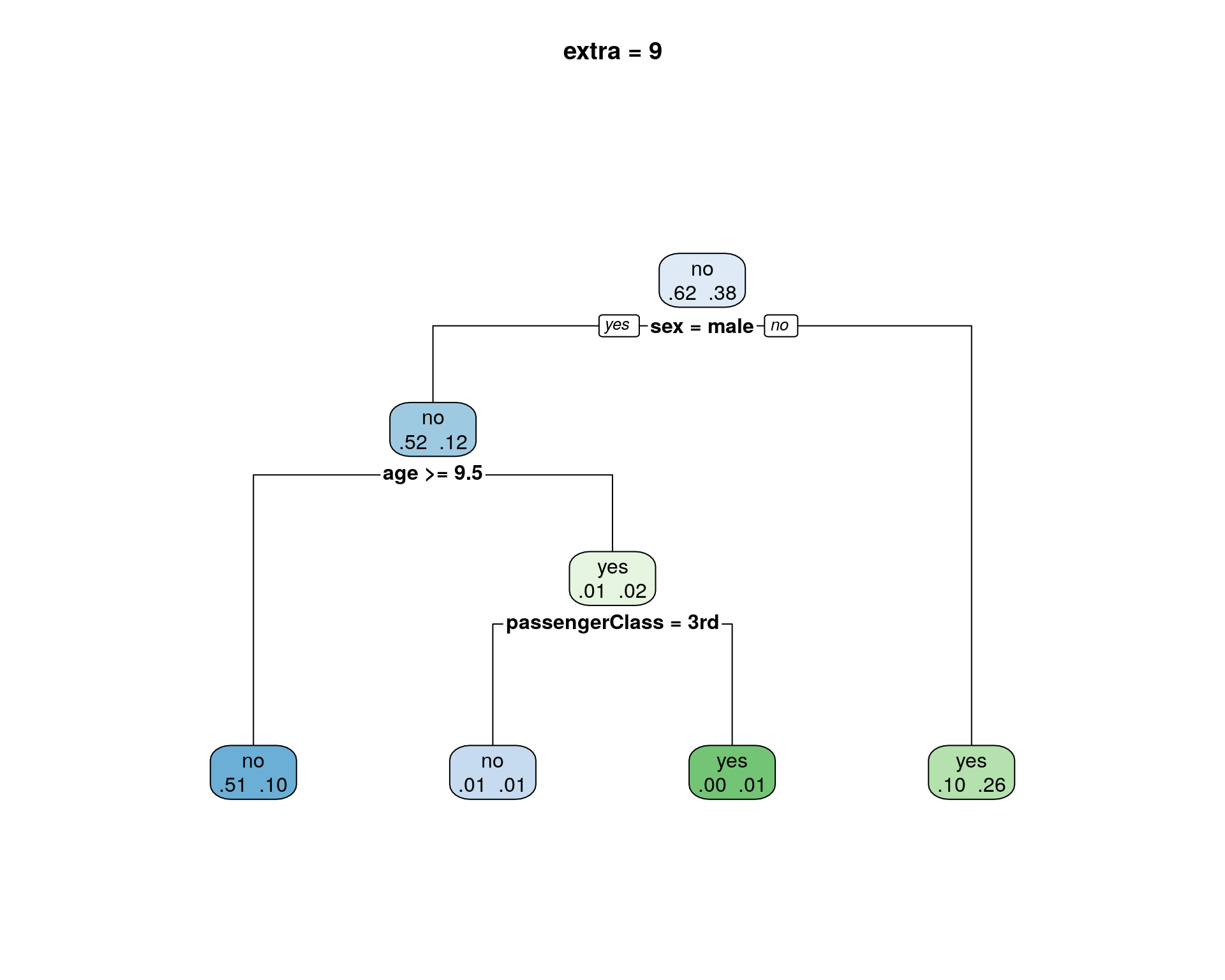
extra = 10
New in version 2.2.0. Class models: Like 9 but display the probability of the second class only. Useful for binary responses.
dt %>%
  rpart.plot::rpart.plot(extra = 10, main = "extra = 10")
extra = 11
New in version 2.2.0. Class models: Like 10 but don’t display the fitted class.
dt %>%
  rpart.plot::rpart.plot(extra = 11, main = "extra =11")
extra = +100s
Add 100 to any of the above to also display the percentage of observations in the node. For example extra=101 displays the number and percentage of observations in the node. Actually, it’s a weighted percentage using the weights passed to rpart.
dt %>%
  rpart.plot::rpart.plot(extra = 100, main = "extra = 0 +100")
dt %>%
  rpart.plot::rpart.plot(extra = 101, main = "extra = 1 +100")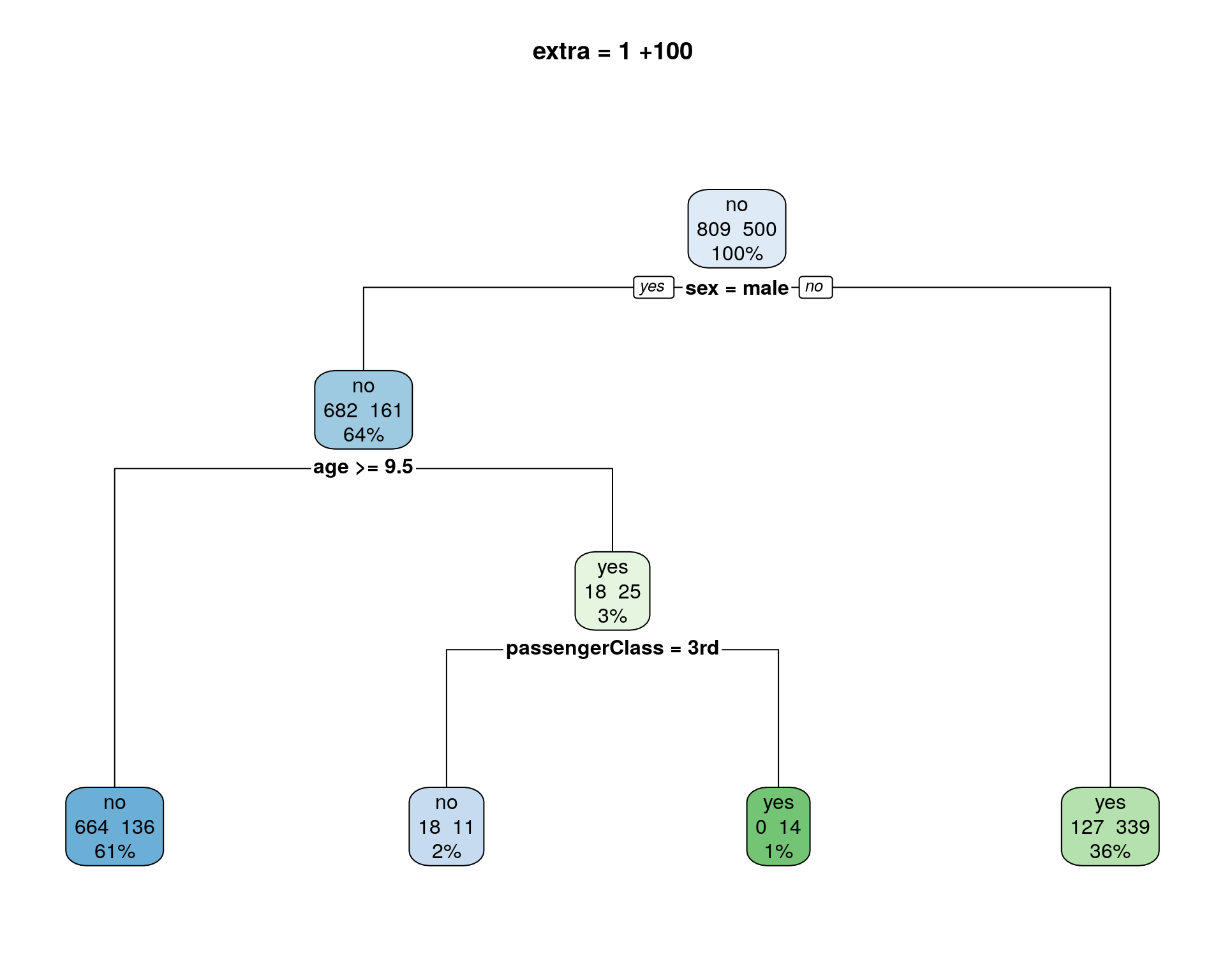
dt %>%
  rpart.plot::rpart.plot(extra = 102, main = "extra = 2 +100")
dt %>%
  rpart.plot::rpart.plot(extra = 103, main = "extra = 3 +100")
dt %>%
  rpart.plot::rpart.plot(extra = 106, main = "extra = 4 +100, for more than tow levels")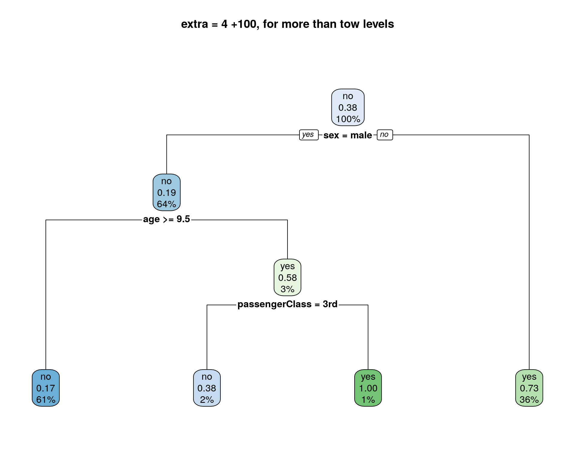
dt %>%
  rpart.plot::rpart.plot(extra = 105, main = "extra = 5 +100")
dt %>%
  rpart.plot::rpart.plot(extra = 106, main = "extra = 106, for binary response")
dt %>%
  rpart.plot::rpart.plot(extra = 107, main = "extra = 7 +100")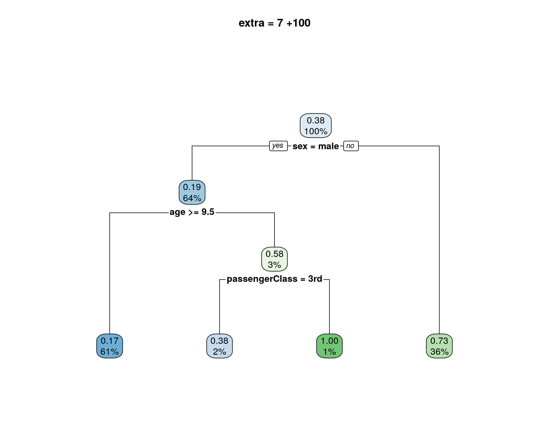
dt %>%
  rpart.plot::rpart.plot(extra = 108, main = "extra = 8 +100")
dt %>%
  rpart.plot::rpart.plot(extra = 109, main = "extra = 9 +100")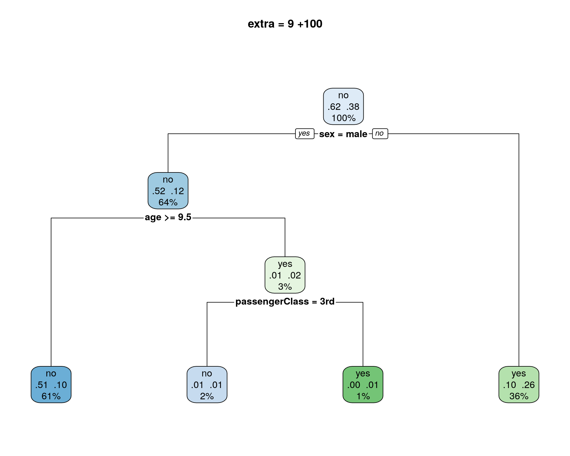
dt %>%
  rpart.plot::rpart.plot(extra = 110, main = "extra = 10 +100")
dt %>%
  rpart.plot::rpart.plot(extra = 111, main = "extra = 11 +100")
おすゝめのオプション
個人的なおすゝめは以下のオプション指定です。枠内の二段階は目的変数であるsurvivedの内訳になります(左側:右側 = no:yes)。内訳の多い方が一段目のラベルになっていることが分かります。
dt %>%
  rpart.plot::rpart.plot(type = 4, extra = 101)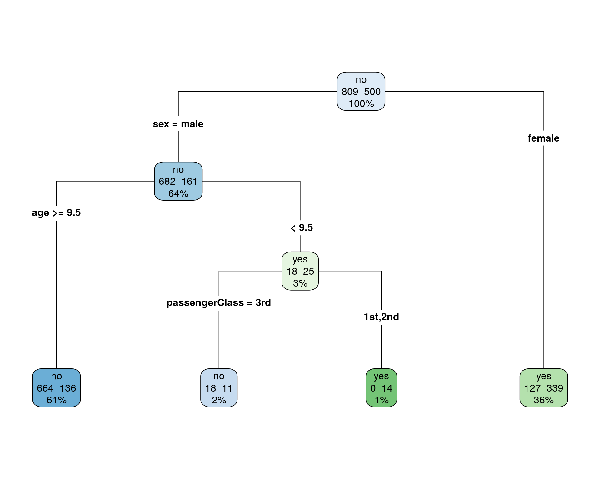
途中のノードの内訳が不要な場合は以下のオプションがおすゝめです。
dt %>%
  rpart.plot::rpart.plot(type = 5, extra = 101)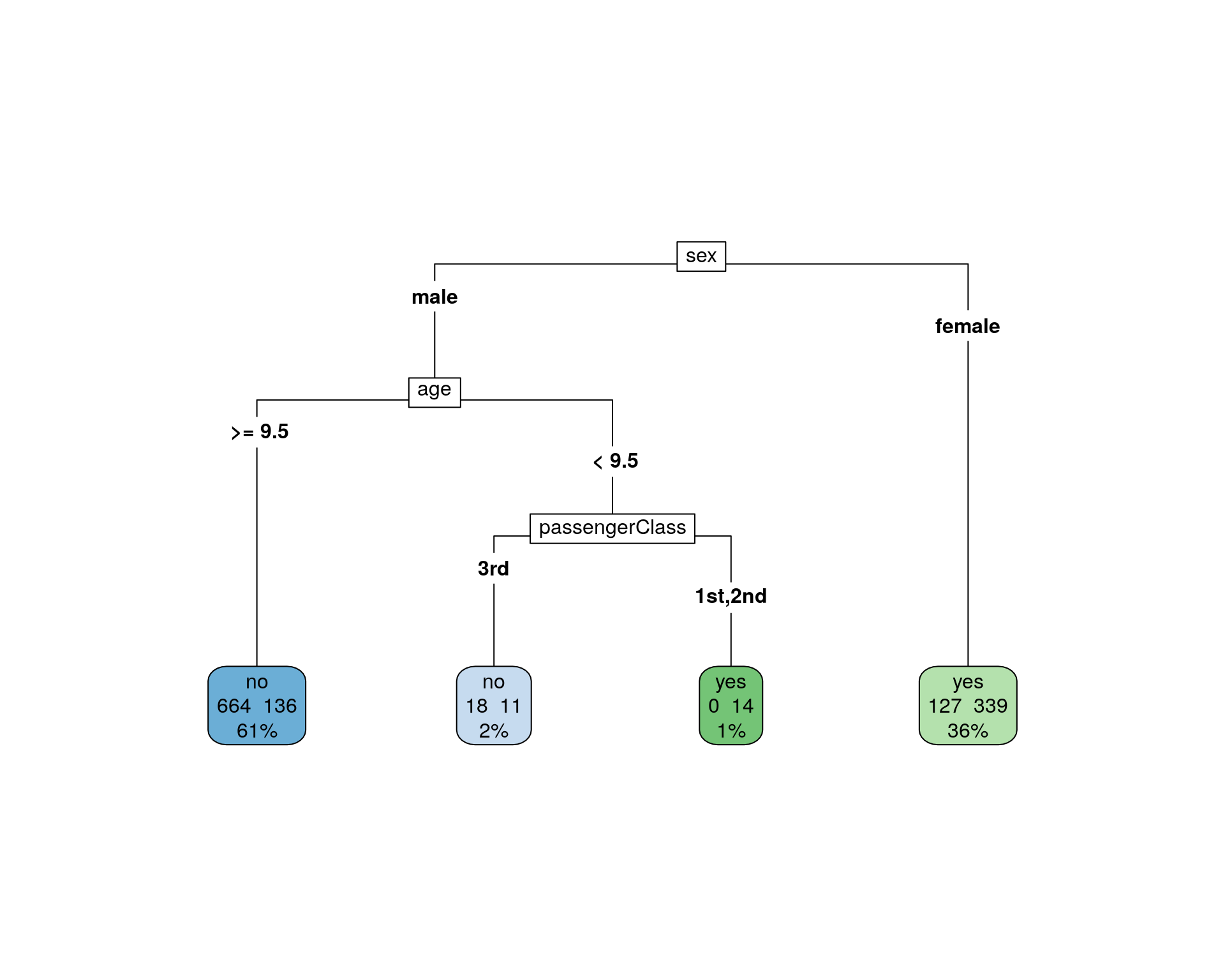
Enjoy!