バグトラッキングシステム(以降、BTS)のチケットデータには様々な情報が記録されており品質分析に使わない手はありません。バグチケットの分析は個々のチケットに対する定性分析を行うことが多いですが、定量分析の面から考えるとバグチケット自体はカテゴリカルデータの塊ですのでODC分析のようにクロス集計を用いる方法が考えられます。ODC分析ではODC分析用のタグに基づいた分析を行いますが、ここではバグチケットにある基本的な情報(項目)を用いた可視化の方法を探って行きます。
Package and Datasets
本ページではR version 3.4.4 (2018-03-15)の標準パッケージ以外に以下の追加パッケージを用いています。
| Package | Version | Description |
|---|---|---|
| tidyverse | 1.2.1 | Easily Install and Load the ‘Tidyverse’ |
| girdExtra | 2.3 | Miscellaneous Functions for “Grid” Graphics |
また、本ページでは以下のデータセットを用いています。
| Dataset | Package | Version | Description |
|---|---|---|---|
| redmine | N/A | N/A | Redmine Issues |
バグチケットは Redmine が公開しているRedmine自体のバグチケットを用います。RedmineはGPL v2ライセンスの下で提供されているオープンソースのプロジェクト管理ソフトウェアです。上表のリンク先でチケットを公開していますが、一度に50レコードまでしかダウンロードできないため事前にこちらで取得したレコードをデータフレーム形式にまとめたものを利用しています。なお、RedmineはREST APIを提供しておりJSON形式でチケット情報取得が可能ですが、REST APIは一度に25件しかチケット情報を取得できない点に注意してください。
チケット情報のインポート
前述のように今回は事前に整理したデータフレーム形式のチケット情報を用いますが、実際にはBTSのAPI機能やBTSのDBMSから直接データを取得することをおすゝめします。直接取得できない場合は、今回のようにCSVファイルへエクスポートするなどの方法を取ってください。
チケットの項目
今回用いるRedmineのバグチケットの項目を簡単に説明してます。基本的な項目のみが用意されています。実際は因子型になっている項目をここでは文字型として扱っている点に注意してください。
| 項目 | 概要 | データ型 |
|---|---|---|
| # | 識別番号(Primary Key) | 整数型 |
| プロジェクト | 属するプロジェクト | 文字型(因子型) |
| トラッカー | 大分類 | 文字型(因子型) |
| 親チケット | 親子関係を定義したい場合に用いる | 文字型 |
| ステータス | 対応状況 | 文字型(因子型) |
| 優先度 | 対応優先度 | 文字型(因子型) |
| 題名 | タイトル | 文字型 |
| 作成者 | 作成者 | 文字型(因子型) |
| 担当者 | 対応担当者 | 文字型(因子型) |
| 更新日 | 更新日時 | 日時型(POSIXct) |
| カテゴリ | 分類(任意に利用設定できる) | 文字型(因子型) |
| 対象バージョン | チケット対処したバージョン | 文字型 |
| 開始日 | 対応を開始した日 | 日付型 |
| 期日 | 対応予定期間 | 日付型 |
| 予定工数 | 対応予定工数 | 数値型 |
| 進捗率 | 対応の進捗率 | 数値型(%表記) |
| 作成日 | 作成日時 | 日時型(POSIXct) |
| 終了日 | 対応完了日時 | 日時型(POSIXct) |
| 関連するチケット | 関係するチケット番号 | 文字型 |
| Resolution | 解決結果(非標準) | 文字型(因子型) |
| Affected version | 影響のあるバージョン | 文字型 |
| 説明 | 詳細 | 文字型 |
チケットデータ
実際のデータは以下のような四千レコード弱のデータです。
(redmine <- "../../static/data/redmine.csv" %>%
readr::read_csv(local = locale(encoding = "UTF-8")))## # A tibble: 3,826 x 22
## `#` プロジェクト トラッカー 親チケット ステータス 優先度 題名 作成者
## <int> <chr> <chr> <chr> <chr> <chr> <chr> <chr>
## 1 28967 Redmine Defect <NA> New Normal coul… jiang…
## 2 28953 Redmine Defect <NA> New Normal Issu… Andr?…
## 3 28951 Redmine Defect <NA> New Normal Cann… L?szl…
## 4 28946 Redmine Defect <NA> New Normal If a… Mariu…
## 5 28943 Redmine Patch <NA> New Low Remo… Sho H…
## 6 28940 Redmine Patch <NA> New Normal redu… Pavel…
## 7 28939 Redmine Patch <NA> Closed Normal repl… Pavel…
## 8 28934 Redmine Patch <NA> New Normal [Rai… Pavel…
## 9 28933 Redmine Patch <NA> New Normal Migr… Pavel…
## 10 28932 Redmine Patch <NA> Closed Normal [Rai… Pavel…
## # ... with 3,816 more rows, and 14 more variables: 担当者 <chr>,
## # 更新日 <dttm>, カテゴリ <chr>, 対象バージョン <chr>, 開始日 <date>,
## # 期日 <chr>, 予定工数 <chr>, 進捗率 <int>, 作成日 <dttm>,
## # 終了日 <dttm>, 関連するチケット <chr>, Resolution <chr>, `Affected
## # version` <chr>, 説明 <chr>
分析のための前処理
分析に必要な前処理を行っておきます。作成日と終了日のデータは実際は日時データになっていますので日データに変換して、必要な項目のみを抽出しておきます。
(x <- redmine %>%
  dplyr::select(no = `#`, tracker = `トラッカー`, status = `ステータス`,
                priority = `優先度`, category = `カテゴリ`,
                version = `対象バージョン`, affected = `Affected version`,
                open = `作成日`, close = `終了日`, subject = `題名`,
                assignee = `担当者`) %>%
dplyr::mutate(open = lubridate::date(open), close = lubridate::date(close)))## # A tibble: 3,826 x 11
## no tracker status priority category version affected open
## <int> <chr> <chr> <chr> <chr> <chr> <chr> <date>
## 1 28967 Defect New Normal REST API <NA> <NA> 2018-06-06
## 2 28953 Defect New Normal Issues <NA> 3.4.5 2018-06-05
## 3 28951 Defect New Normal Issues <NA> 3.4.5 2018-06-05
## 4 28946 Defect New Normal Issues Candid… 3.4.5 2018-06-04
## 5 28943 Patch New Low Documen… 4.1.0 <NA> 2018-06-04
## 6 28940 Patch New Normal Perform… Candid… <NA> 2018-06-04
## 7 28939 Patch Closed Normal Perform… <NA> <NA> 2018-06-04
## 8 28934 Patch New Normal Perform… <NA> <NA> 2018-06-02
## 9 28933 Patch New Normal Gems su… Candid… <NA> 2018-06-01
## 10 28932 Patch Closed Normal Code cl… <NA> <NA> 2018-06-01
## # ... with 3,816 more rows, and 3 more variables: close <date>,
## # subject <chr>, assignee <chr>
また、statusやpriorityのようなデータは順位尺度として扱えるように順序付きの因子に変換しておきます。
x <- x %>%
  dplyr::mutate(status = ordered(status, levels = c("New", "Needs feedback",
                                            "Confirmed", "Resolved", "Closed",
                                            "Reopened"))) %>%
  dplyr::mutate(priority = ordered(priority, levels = c("Low", "Normal",
                                                        "High", "Urgent")))
データの概要は以下の通りです。
summary(x) no tracker status priority
Min. :13710 Length:3826 New : 680 Low : 108
1st Qu.:16722 Class :character Needs feedback: 160 Normal:3435
Median :20346 Mode :character Confirmed : 29 High : 203
Mean :20647 Resolved : 13 Urgent: 80
3rd Qu.:24342 Closed :2934
Max. :28967 Reopened : 10
category version affected
Length:3826 Length:3826 Length:3826
Class :character Class :character Class :character
Mode :character Mode :character Mode :character
open close subject
Min. :2013-04-08 Min. :2010-07-19 Length:3826
1st Qu.:2014-04-19 1st Qu.:2014-07-21 Class :character
Median :2015-07-16 Median :2015-08-31 Mode :character
Mean :2015-08-17 Mean :2015-09-10
3rd Qu.:2016-11-13 3rd Qu.:2016-11-18
Max. :2018-06-06 Max. :2018-06-06
NA's :870
assignee
Length:3826
Class :character
Mode :character
集計による可視化
データフレームに対する集計を行うにはdplyr::group_by関数+dplyr::summarise関数またはdplyr::count関数を用いるのが便利です。
なお、以下の二つのコードは共にdataに含まれるkey変数の水準毎に個数を数えるもので結果は等価になります。
dplyr::group_by(data, key) %>%
dplyr::summarise(n = n())dplyr::count(data, kye)
単純集計
単純集計は一つの変数に対して集計を行います。単純集計はdplyr::count関数で処理することができます。
dplyr::count(x, key)
単純集計を可視化するには比率が見やすい円グラフや積み上げ棒グラフが便利です。
Tracker
x %>%
dplyr::count(tracker)## # A tibble: 2 x 2
## tracker n
## <chr> <int>
## 1 Defect 2868
## 2 Patch 958x %>%
dplyr::count(tracker) %>%
ggplot2::ggplot(ggplot2::aes(x = "tracker", y = n, fill = tracker)) +
ggplot2::geom_bar(stat = "identity", width = 1, alpha = 0.75) +
ggplot2::coord_polar(theta = "y", direction = 1) +
ggplot2::guides(fill = guide_legend(reverse = TRUE))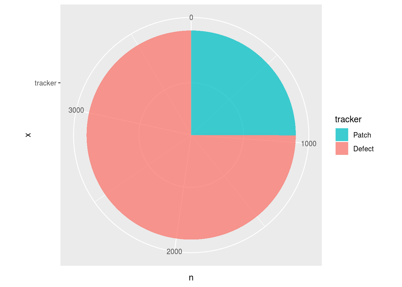
Status
x %>%
dplyr::count(status)## # A tibble: 6 x 2
## status n
## <ord> <int>
## 1 New 680
## 2 Needs feedback 160
## 3 Confirmed 29
## 4 Resolved 13
## 5 Closed 2934
## 6 Reopened 10x %>%
dplyr::count(status) %>%
ggplot2::ggplot(ggplot2::aes(x = "status", y = n, fill = status)) +
ggplot2::geom_bar(stat = "identity", width = 1, alpha = 0.75) +
ggplot2::coord_polar(theta = "y", direction = 1) +
ggplot2::guides(fill = guide_legend(reverse = TRUE))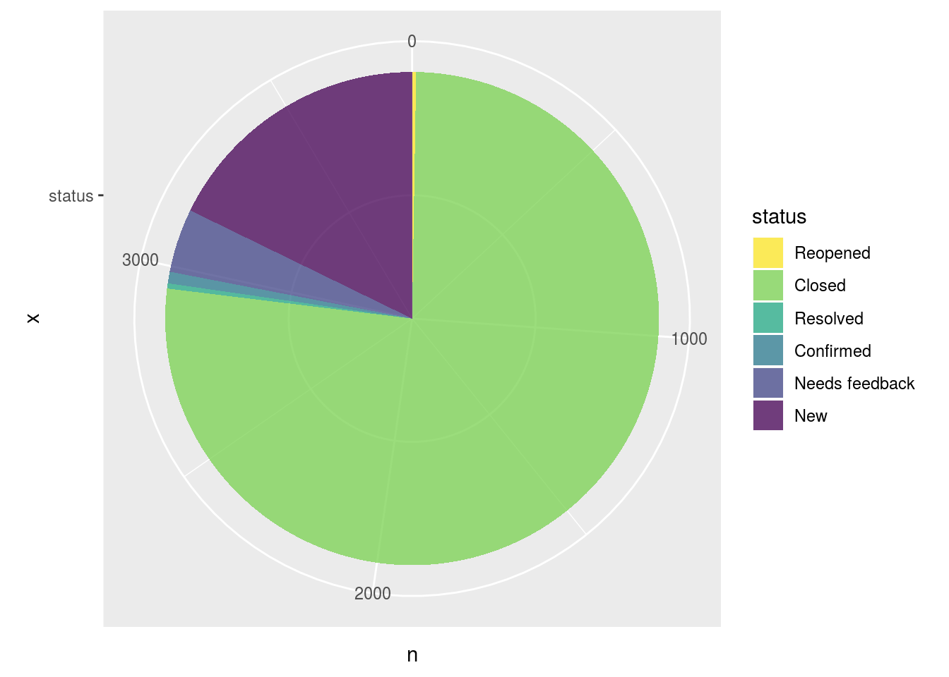
Priority
x %>%
dplyr::count(priority)## # A tibble: 4 x 2
## priority n
## <ord> <int>
## 1 Low 108
## 2 Normal 3435
## 3 High 203
## 4 Urgent 80x %>%
dplyr::count(priority) %>%
ggplot2::ggplot(ggplot2::aes(x = "priority", y = n, fill = priority)) +
ggplot2::geom_bar(stat = "identity", width = 1, alpha = 0.75) +
ggplot2::coord_polar(theta = "y", direction = 1) +
ggplot2::guides(fill = guide_legend(reverse = TRUE))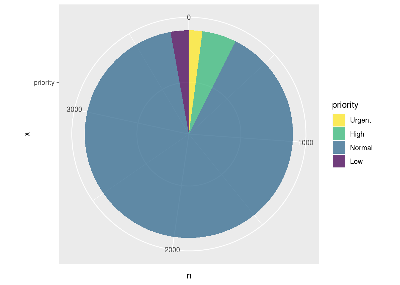
Category
カテゴリ数が多い場合、円グラフや積み上げ棒グラフによる可視化はあまり好ましくありません。
x %>%
dplyr::count(category)## # A tibble: 56 x 2
## category n
## <chr> <int>
## 1 Accounts / authentication 58
## 2 Activity view 20
## 3 Administration 54
## 4 Attachments 90
## 5 Calendar 9
## 6 Code cleanup/refactoring 126
## 7 Core Plugins 3
## 8 Custom fields 114
## 9 Database 85
## 10 Documentation 60
## # ... with 46 more rowsx %>%
dplyr::count(category) %>%
ggplot2::ggplot(ggplot2::aes(x = "category", y = n, fill = category)) +
ggplot2::geom_bar(stat = "identity", width = 1, alpha = 0.75) +
ggplot2::coord_polar(theta = "y", direction = 1) +
ggplot2::guides(fill = guide_legend(reverse = TRUE))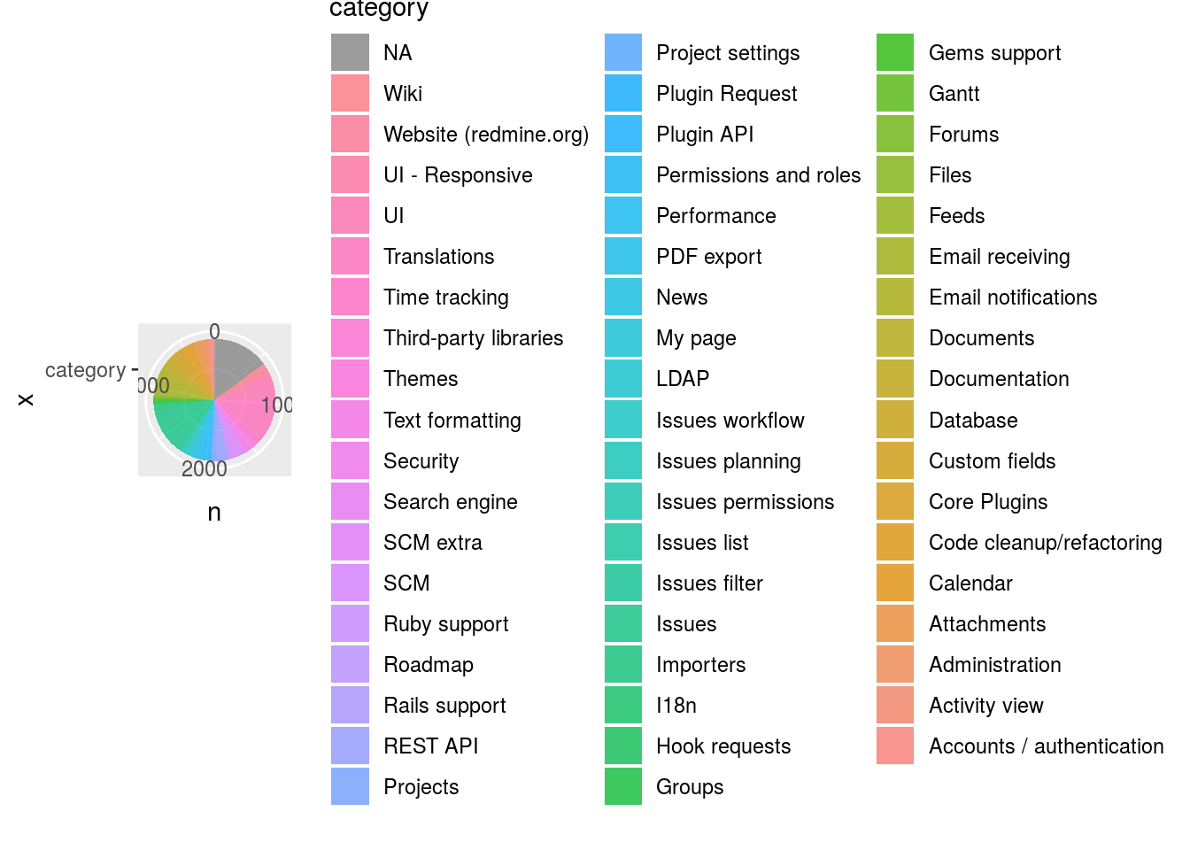
Version
x %>%
dplyr::count(version)## # A tibble: 72 x 2
## version n
## <chr> <int>
## 1 2.3.1 3
## 2 2.3.2 20
## 3 2.3.3 17
## 4 2.3.4 13
## 5 2.4.0 48
## 6 2.4.1 7
## 7 2.4.2 12
## 8 2.4.3 8
## 9 2.4.4 4
## 10 2.4.6 5
## # ... with 62 more rowsx %>%
dplyr::count(version) %>%
dplyr::filter(!is.na(version)) %>%
ggplot2::ggplot(ggplot2::aes(x = "version", y = n, fill = version)) +
ggplot2::geom_bar(stat = "identity", width = 1, alpha = 0.75) +
ggplot2::coord_polar(theta = "y", direction = 1) +
ggplot2::guides(fill = guide_legend(reverse = TRUE))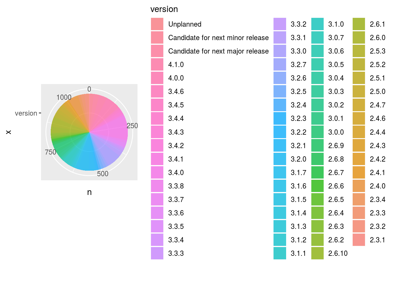
Affected
x %>%
dplyr::count(affected)## # A tibble: 91 x 2
## affected n
## <chr> <int>
## 1 0.8.2 1
## 2 0.8.5 1
## 3 0.8.7 1
## 4 0.9.4 1
## 5 0.9.6 2
## 6 1.0.1 2
## 7 1.0.4 1
## 8 1.1.2 1
## 9 1.1.3 2
## 10 1.2.0 1
## # ... with 81 more rowsx %>%
dplyr::count(affected) %>%
dplyr::filter(!is.na(affected)) %>%
ggplot2::ggplot(ggplot2::aes(x = "affected", y = n, fill = affected)) +
ggplot2::geom_bar(stat = "identity", width = 1, alpha = 0.75) +
ggplot2::coord_polar(theta = "y", direction = 1) +
ggplot2::guides(fill = guide_legend(reverse = TRUE))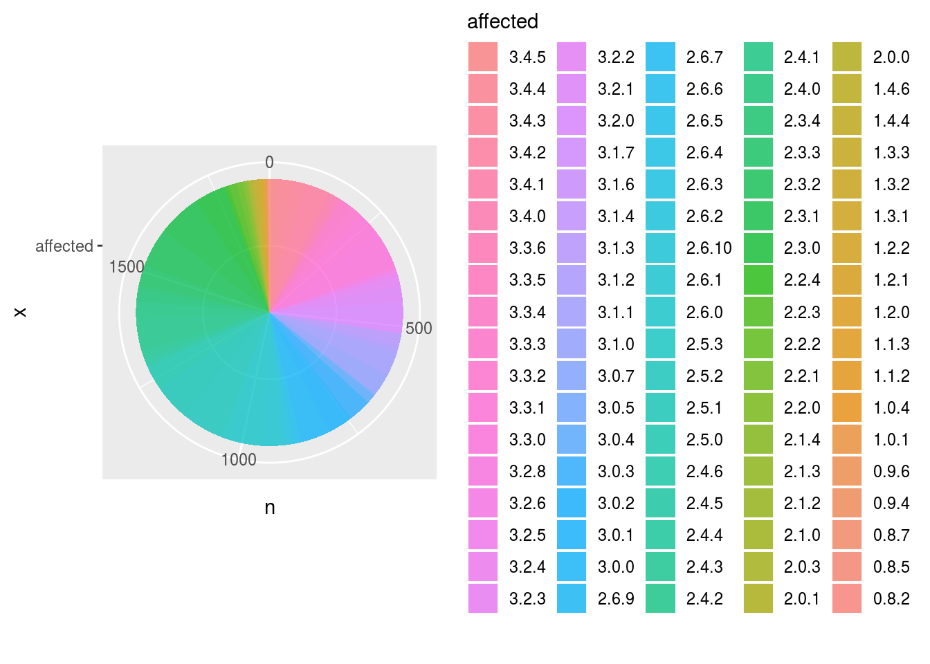
Open
ggplot2パッケージでは日付は連続量として扱われるため円グラフで表現するのはおすゝめできません。
x %>%
dplyr::count(open)## # A tibble: 1,466 x 2
## open n
## <date> <int>
## 1 2013-04-08 4
## 2 2013-04-09 6
## 3 2013-04-10 4
## 4 2013-04-11 5
## 5 2013-04-12 8
## 6 2013-04-14 3
## 7 2013-04-15 2
## 8 2013-04-16 5
## 9 2013-04-17 5
## 10 2013-04-18 3
## # ... with 1,456 more rowsx %>%
dplyr::count(open) %>%
ggplot2::ggplot(ggplot2::aes(x = "open", y = n, fill = open)) +
ggplot2::geom_bar(stat = "identity", width = 1, alpha = 0.75) +
ggplot2::coord_polar(theta = "y", direction = 1) +
ggplot2::guides(fill = guide_legend(reverse = TRUE))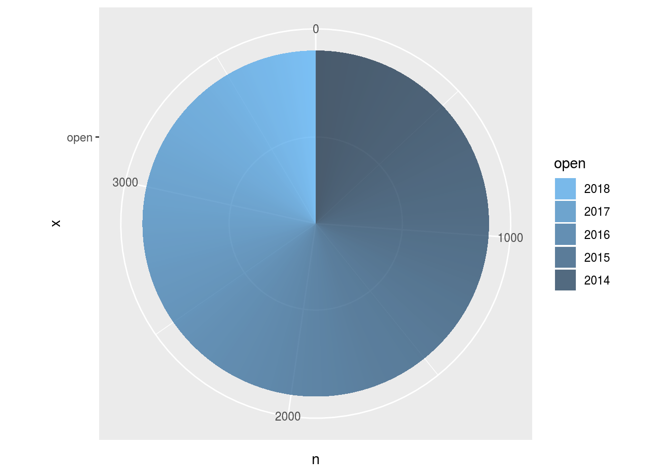
クロス集計
単純集計では見えにくい傾向はクロス集計を行いことで見えてくることもあります。クロス集計はdplyr::count関数またはdplyr::group_by関数に複数の変数を指定し、tidyr::spread関数で変形することで簡単にクロス集計表が作成できます。
dplyr::count(x, key1, key2) %>%
  tidyr::spread(key = key1, value = n)
なお、クロス集計を可視化するにはヒートマップ(ggplot2::gemo_tile)や同心円グラフが便利です。
Tracker and Status
x %>%
  dplyr::count(tracker, status) %>%
tidyr::spread(key = tracker, value = n)## # A tibble: 6 x 3
## status Defect Patch
## <ord> <int> <int>
## 1 New 504 176
## 2 Needs feedback 144 16
## 3 Confirmed 29 NA
## 4 Resolved 10 3
## 5 Closed 2174 760
## 6 Reopened 7 3x %>%
dplyr::count(tracker, status) %>%
ggplot2::ggplot(ggplot2::aes(x = tracker, y = status, fill = n)) +
ggplot2::geom_tile() +
ggplot2::scale_fill_gradient(low = "lightyellow", high = "red") +
ggplot2::geom_text(ggplot2::aes(label = n)) +
ggplot2::theme_bw()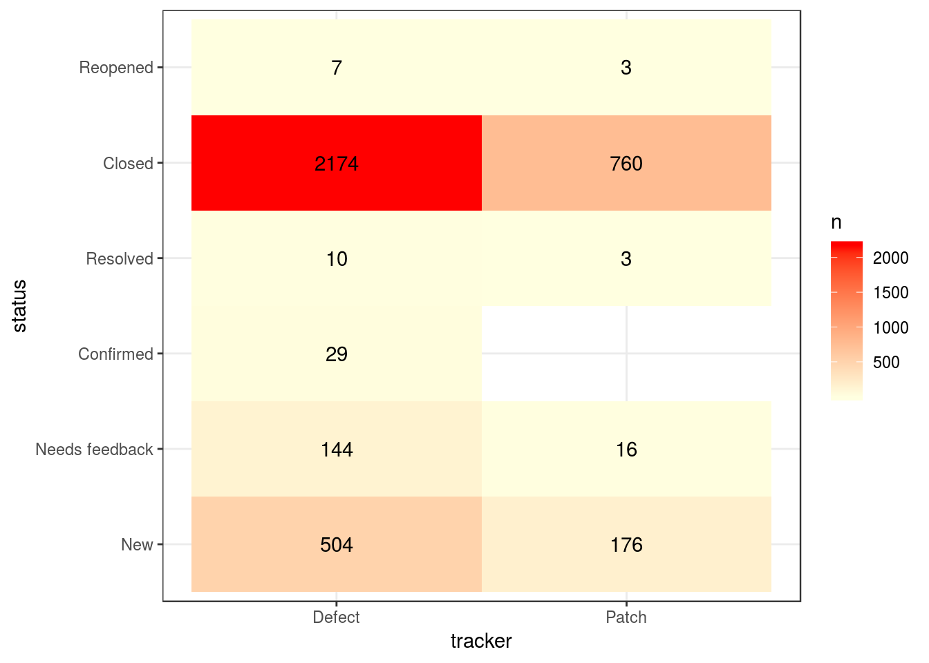
x %>%
  dplyr::count(tracker, status) %>%
  ggplot2::ggplot(ggplot2::aes(x = tracker, y = n, fill = status)) +
    ggplot2::geom_bar(stat = "identity", alpha = 0.75) +
    ggplot2::coord_polar(theta = "y", direction = 1) +
    ggplot2::theme_bw() +
    ggplot2::guides(fill = guide_legend(reverse = TRUE))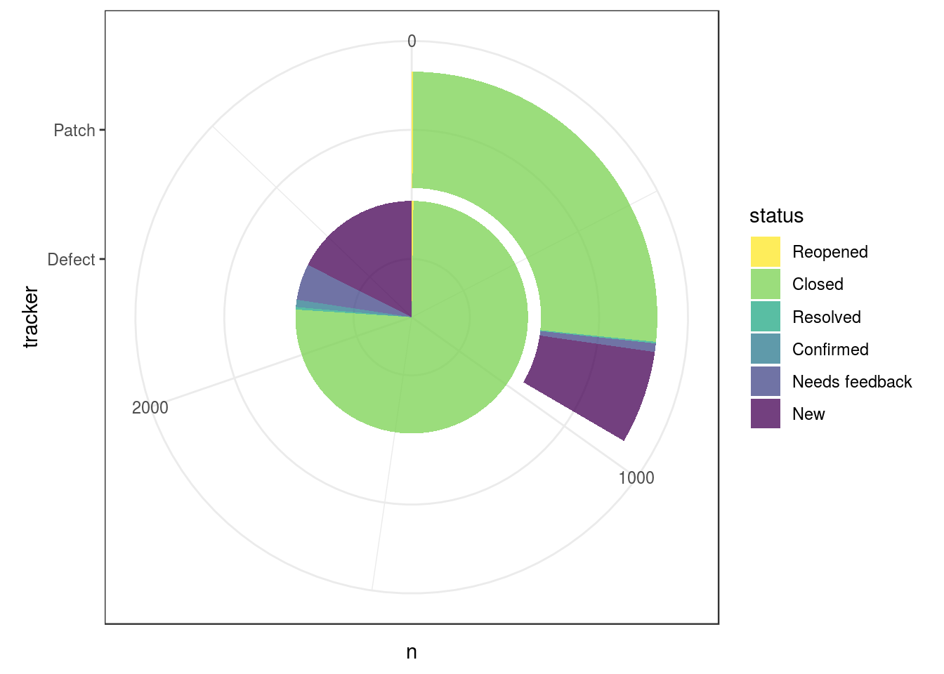
Tracker and Priority
大半のチケットがステータスがClosedな対応が完了しているチケットですので、Closedを除くチケットに対する優先度を見て見ます。
x %>%
  dplyr::filter(status != "Closed") %>%
  dplyr::count(tracker, priority) %>%
tidyr::spread(key = tracker, value = n)## # A tibble: 4 x 3
## priority Defect Patch
## <ord> <int> <int>
## 1 Low 28 2
## 2 Normal 606 193
## 3 High 50 3
## 4 Urgent 10 NAx %>%
dplyr::filter(status != "Closed") %>%
dplyr::count(tracker, priority) %>%
ggplot2::ggplot(ggplot2::aes(x = tracker, y = priority, fill = n)) +
ggplot2::geom_tile() +
ggplot2::scale_fill_gradient(low = "lightyellow", high = "red") +
ggplot2::geom_text(ggplot2::aes(label = n)) +
ggplot2::theme_bw()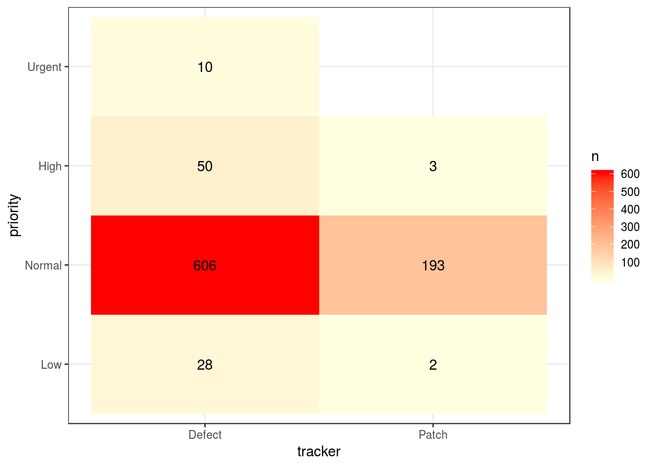
x %>%
  dplyr::filter(status != "Closed") %>%
  dplyr::count(tracker, priority) %>%
  ggplot2::ggplot(ggplot2::aes(x = tracker, y = n, fill = priority)) +
    ggplot2::geom_bar(stat = "identity", alpha = 0.75) +
    ggplot2::coord_polar(theta = "y", direction = 1) +
    ggplot2::theme_bw() +
    ggplot2::guides(fill = guide_legend(reverse = TRUE))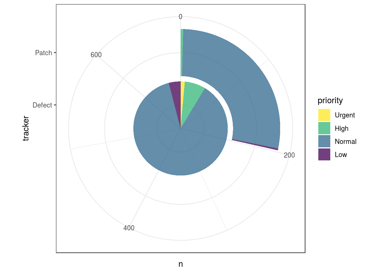
Priority and Status
Defectチケット
x %>%
  dplyr::filter(status != "Closed" & tracker == "Defect") %>%
  dplyr::count(priority, status) %>%
tidyr::spread(key = priority, value = n)## # A tibble: 5 x 5
## status Low Normal High Urgent
## <ord> <int> <int> <int> <int>
## 1 New 25 435 37 7
## 2 Needs feedback 3 131 8 2
## 3 Confirmed NA 27 2 NA
## 4 Resolved NA 8 1 1
## 5 Reopened NA 5 2 NAx %>%
dplyr::filter(status != "Closed" & tracker == "Defect") %>%
dplyr::count(priority, status) %>%
ggplot2::ggplot(ggplot2::aes(x = status, y = priority, fill = n)) +
ggplot2::geom_tile() +
ggplot2::scale_fill_gradient(low = "lightyellow", high = "red") +
ggplot2::geom_text(ggplot2::aes(label = n)) +
ggplot2::theme_bw()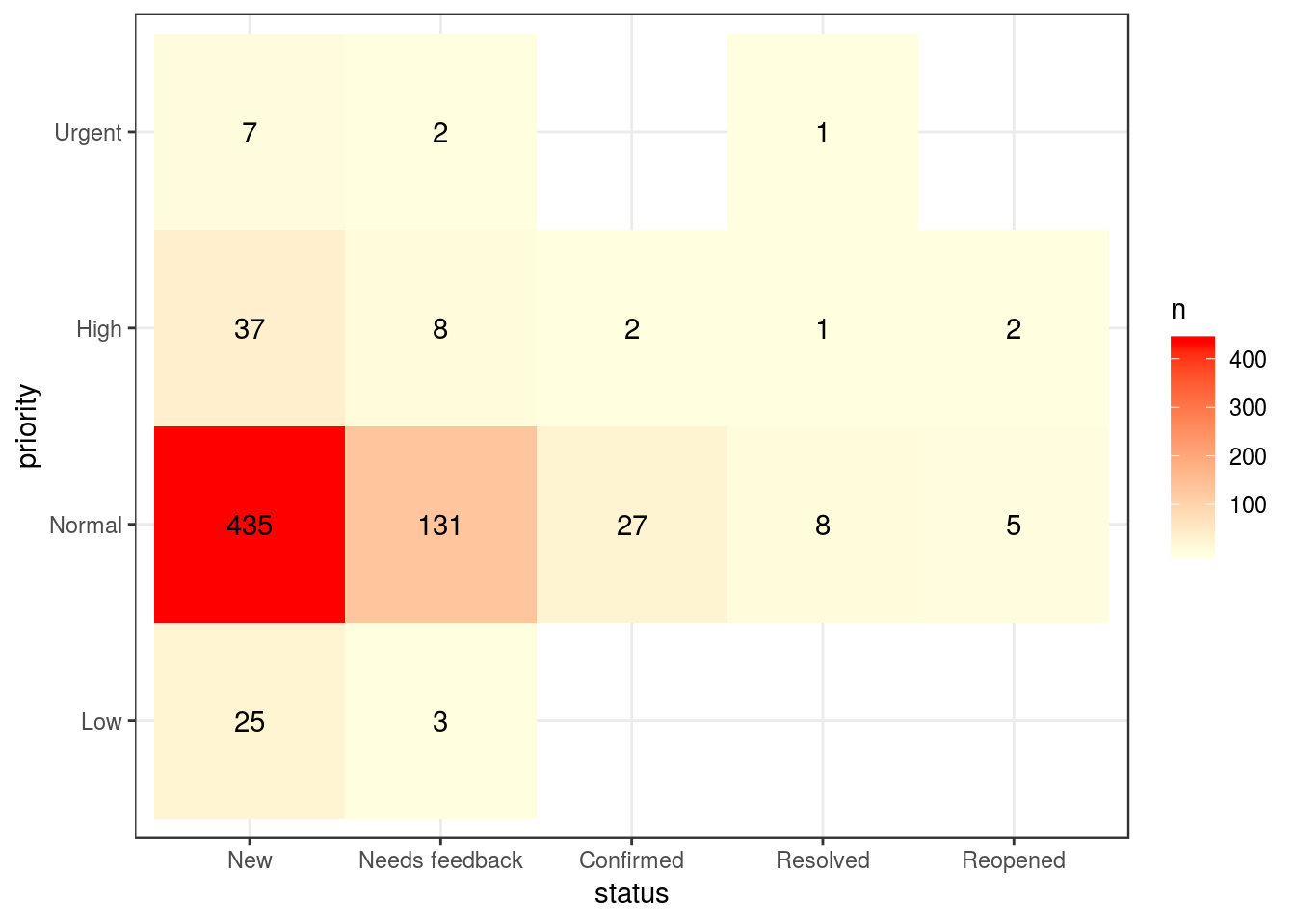
x %>%
  dplyr::filter(status != "Closed" & tracker == "Defect") %>%
  dplyr::count(priority, status) %>%
  ggplot2::ggplot(ggplot2::aes(x = priority, y = n, fill = status)) +
    ggplot2::geom_bar(stat = "identity", alpha = 0.75) +
    ggplot2::coord_polar(theta = "y", direction = 1) +
    ggplot2::theme_bw() +
    ggplot2::guides(fill = guide_legend(reverse = TRUE))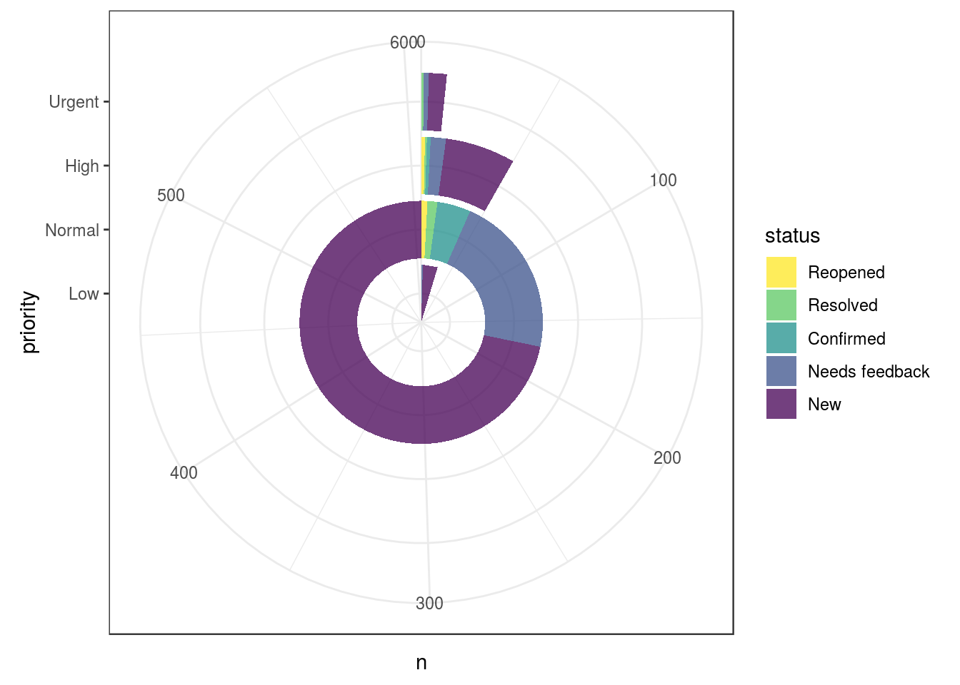
Patchチケット
x %>%
  dplyr::filter(status != "Closed" & tracker == "Patch") %>%
  dplyr::count(priority, status) %>%
tidyr::spread(key = priority, value = n)## # A tibble: 4 x 4
## status Low Normal High
## <ord> <int> <int> <int>
## 1 New 2 171 3
## 2 Needs feedback NA 16 NA
## 3 Resolved NA 3 NA
## 4 Reopened NA 3 NAx %>%
dplyr::filter(status != "Closed" & tracker == "Patch") %>%
dplyr::count(priority, status) %>%
ggplot2::ggplot(ggplot2::aes(x = status, y = priority, fill = n)) +
ggplot2::geom_tile() +
ggplot2::scale_fill_gradient(low = "lightyellow", high = "red") +
ggplot2::geom_text(ggplot2::aes(label = n)) +
ggplot2::theme_bw()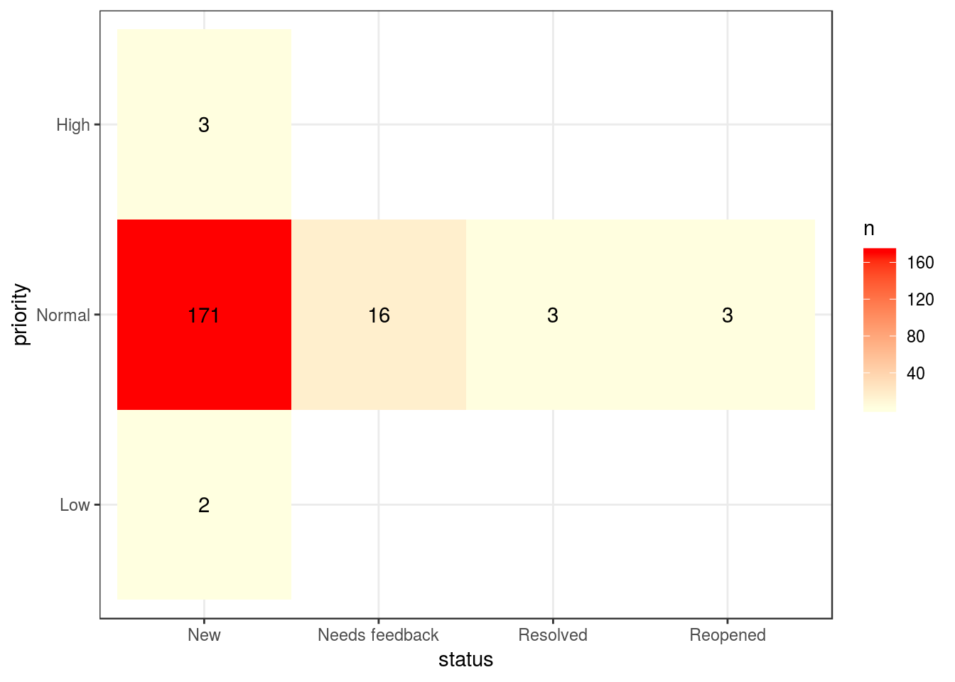
x %>%
  dplyr::filter(status != "Closed" & tracker == "Patch") %>%
  dplyr::count(priority, status) %>%
  ggplot2::ggplot(ggplot2::aes(x = priority, y = n, fill = status)) +
    ggplot2::geom_bar(stat = "identity", alpha = 0.75) +
    ggplot2::coord_polar(theta = "y", direction = 1) +
    ggplot2::theme_bw() +
    ggplot2::guides(fill = guide_legend(reverse = TRUE))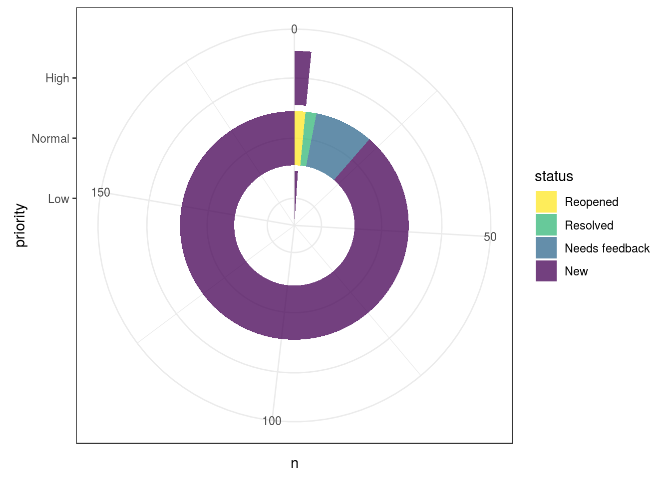
対象レコードの抽出
クロス集計の結果優先度がUrgentであるチケットがあることが分かりましたので、対象が何かを表示させてみます。クロス集計で検索条件が分かっていますので絞り込むだけです。
x %>%
  dplyr::filter(status != "Closed" & tracker == "Defect") %>%
  dplyr::filter(priority == "Urgent") %>%
dplyr::select(no, tracker, status, subject, assignee)## # A tibble: 10 x 5
## no tracker status subject assignee
## <int> <chr> <ord> <chr> <chr>
## 1 28303 Defect New Documentation needs tutorial for ins… <NA>
## 2 28188 Defect New No Access-Control-Allow-Origin <NA>
## 3 27863 Defect New If version is closed or locked subt… <NA>
## 4 18984 Defect Resolved migrate_from_mantis with NoMethodErr… <NA>
## 5 15560 Defect Needs fee… RJS leaking <NA>
## 6 14979 Defect Needs fee… Delete Issues Relation <NA>
## 7 14969 Defect New ActiceSupport::TimeWithZone failed i… <NA>
## 8 14918 Defect New Name with quote displays in ASCII <NA>
## 9 14269 Defect New custom field not displayed but not i… <NA>
## 10 14251 Defect New Redmine email reminders sending 4 em… <NA>
Priority and Category
x %>%
  dplyr::filter(status != "Closed" & tracker == "Defect") %>%
  dplyr::count(category, priority) %>%
tidyr::spread(key = priority, value = n)## # A tibble: 50 x 5
## category Low Normal High Urgent
## <chr> <int> <int> <int> <int>
## 1 Accounts / authentication NA 11 1 1
## 2 Activity view 1 3 NA NA
## 3 Administration NA 7 2 NA
## 4 Attachments 2 14 NA NA
## 5 Calendar NA 2 NA NA
## 6 Code cleanup/refactoring NA 4 1 NA
## 7 Custom fields NA 33 1 NA
## 8 Database 1 21 2 NA
## 9 Documentation 1 9 NA 1
## 10 Documents NA 1 NA NA
## # ... with 40 more rowsx %>%
dplyr::filter(status != "Closed" & tracker == "Defect") %>%
dplyr::count(category, priority) %>%
ggplot2::ggplot(ggplot2::aes(x = category, y = priority, fill = n)) +
ggplot2::geom_tile() +
ggplot2::scale_fill_gradient(low = "lightyellow", high = "red") +
ggplot2::theme_bw() +
ggplot2::coord_flip()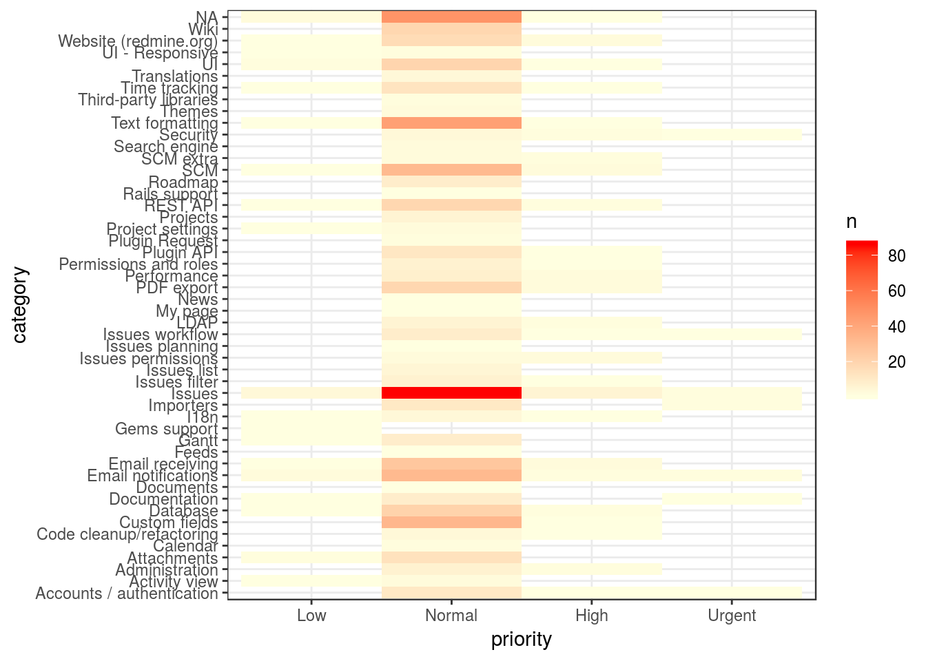
x %>%
  dplyr::filter(status != "Closed" & tracker == "Defect") %>%
  dplyr::count(category, priority) %>%
  ggplot2::ggplot(ggplot2::aes(x = category, y = n, fill = priority)) +
    ggplot2::geom_bar(stat = "identity", alpha = 0.75) +
    ggplot2::coord_polar(theta = "x", direction = 1) +
    ggplot2::theme_bw() +
    ggplot2::guides(fill = guide_legend(reverse = TRUE))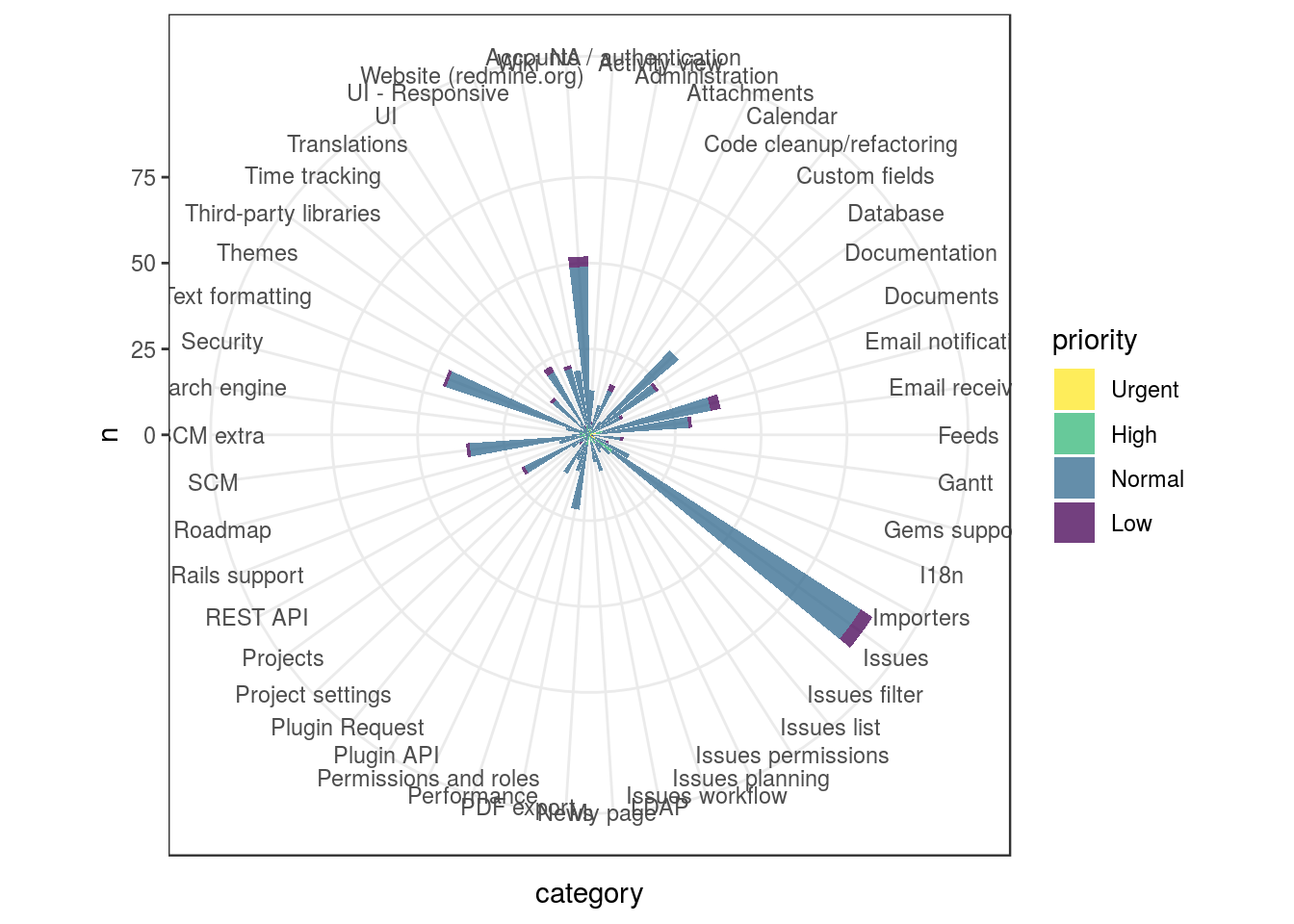
Priority and Assignee
x %>%
  dplyr::filter(status != "Closed" & tracker == "Defect") %>%
  dplyr::count(priority, assignee) %>%
tidyr::spread(key = priority, value = n)## # A tibble: 7 x 5
## assignee Low Normal High Urgent
## <chr> <int> <int> <int> <int>
## 1 Gregor Schmidt NA 1 NA NA
## 2 Jean-Baptiste Barth NA 1 NA NA
## 3 Jean-Philippe Lang NA 22 3 NA
## 4 Marius BALTEANU NA 3 NA NA
## 5 Mischa The Evil NA 3 NA NA
## 6 Toshi MARUYAMA NA 2 NA NA
## 7 <NA> 28 574 47 10x %>%
dplyr::filter(status != "Closed" & tracker == "Defect") %>%
dplyr::count(priority, assignee) %>%
ggplot2::ggplot(ggplot2::aes(x = assignee, y = priority, fill = n)) +
ggplot2::geom_tile() +
ggplot2::scale_fill_gradient(low = "lightyellow", high = "red") +
ggplot2::theme_bw() +
ggplot2::coord_flip()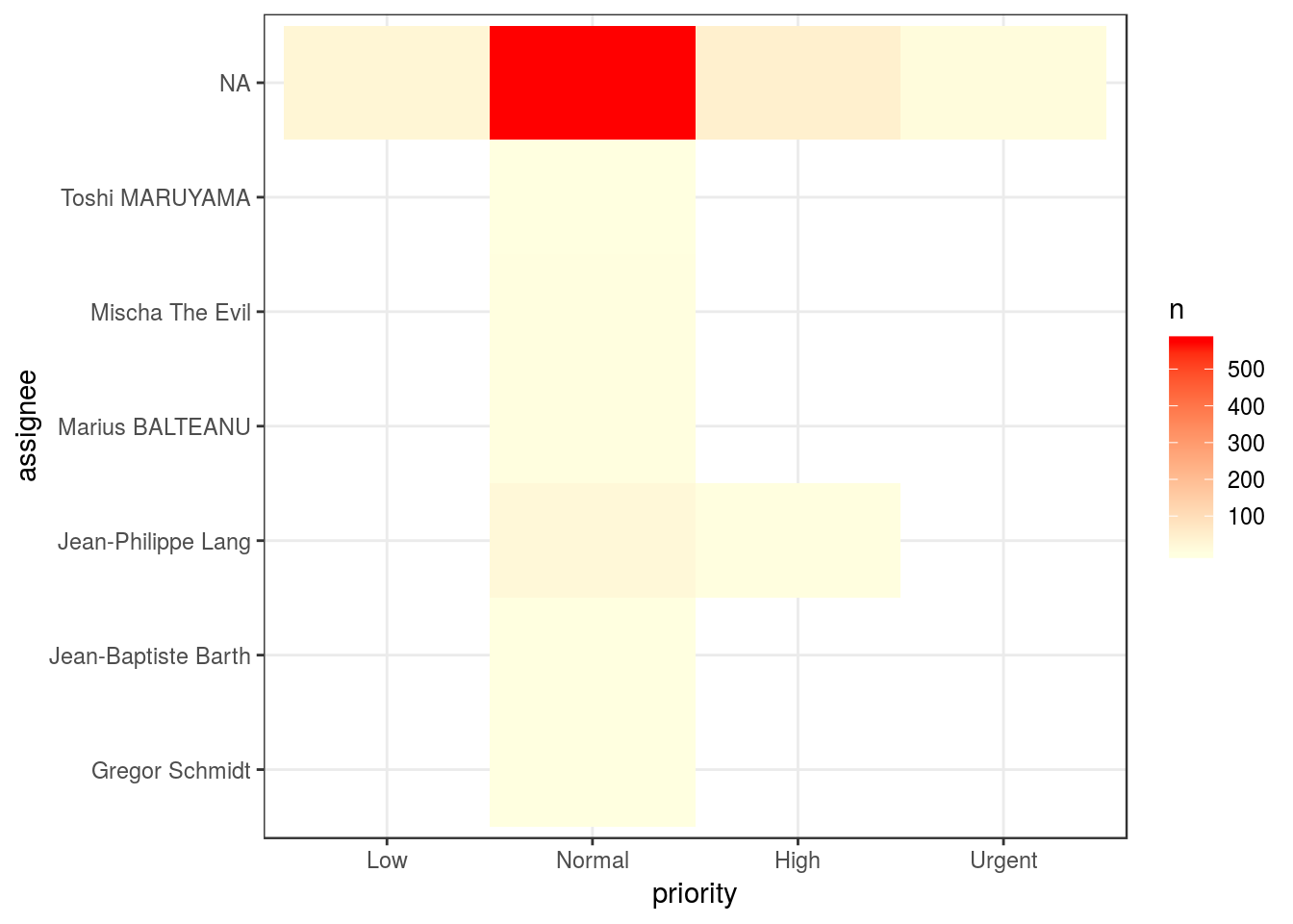
x %>%
  dplyr::filter(status != "Closed" & tracker == "Defect") %>%
  dplyr::count(priority, assignee) %>%
  ggplot2::ggplot(ggplot2::aes(x = priority, y = n, fill = assignee)) +
    ggplot2::geom_bar(stat = "identity", alpha = 0.75) +
    ggplot2::coord_polar(theta = "y", direction = 1) +
    ggplot2::theme_bw() +
    ggplot2::guides(fill = guide_legend(reverse = TRUE))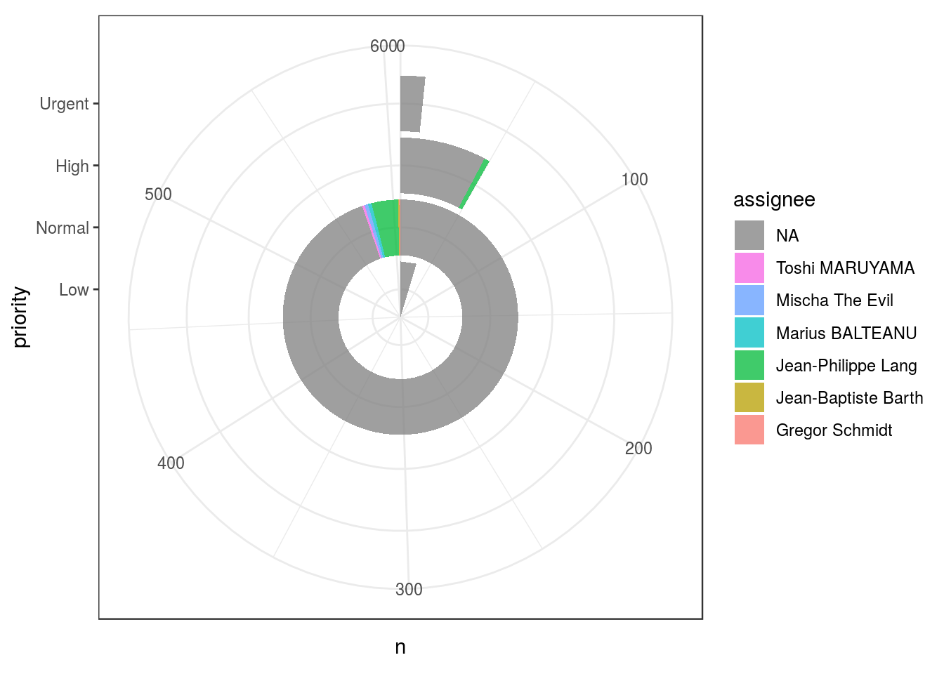
このデータではUrgentなチケットに担当者が割り当てられていないことが分かります。
期間集計
ある一定期間ごとに集計する場合は日時データを日、週、月、四半期、年などに変換し変換後のデータをdplyr::count関数で集計することで期間の変化を確認できるようになります。なお、期間集計は時系列の集計ですので可視化する場合には棒グラフ、折れ線グラフを利用することが多いです。
日次集計
日次で集計する場合は日時の場合はlubridate::date関数で日付に変換しておきます。データがない日は集計対象外となります。稼働が発生していてデータがないのか、稼働が発生していないからデータがないのかで意味が変わってきますので集計の際には注意してください。
起票されたチケットの推移
x %>%
  dplyr::filter(open >= "2018-1-1" & tracker == "Defect") %>%
  dplyr::mutate(flag = ifelse(is.na(open), 0, 1)) %>%
  dplyr::group_by(open) %>%
  dplyr::summarise(ticket = sum(flag)) %>%
  dplyr::arrange(open) %>%
  dplyr::mutate(`累計` = cumsum(ticket),
`前日との差` = ticket - dplyr::lag(ticket))## # A tibble: 98 x 4
## open ticket 累計 前日との差
## <date> <dbl> <dbl> <dbl>
## 1 2018-01-02 1 1 NA
## 2 2018-01-03 5 6 4
## 3 2018-01-04 1 7 -4
## 4 2018-01-05 3 10 2
## 5 2018-01-08 1 11 -2
## 6 2018-01-09 2 13 1
## 7 2018-01-11 1 14 -1
## 8 2018-01-12 2 16 1
## 9 2018-01-13 2 18 0
## 10 2018-01-15 1 19 -1
## # ... with 88 more rowsgg_bar <- x %>%
dplyr::filter(open >= "2018-1-1" & tracker == "Defect") %>%
dplyr::mutate(flag = ifelse(is.na(open), 0, 1)) %>%
dplyr::group_by(open) %>%
dplyr::summarise(ticket = sum(flag)) %>%
dplyr::arrange(open) %>%
dplyr::mutate(`累計` = cumsum(ticket),
`前日との差` = ticket - dplyr::lag(ticket)) %>%
ggplot2::ggplot(ggplot2::aes(x = open)) +
ggplot2::geom_bar(ggplot2::aes(y = ticket), stat = "identity")
gg_line <- x %>%
dplyr::filter(open >= "2018-1-1" & tracker == "Defect") %>%
dplyr::mutate(flag = ifelse(is.na(open), 0, 1)) %>%
dplyr::group_by(open) %>%
dplyr::summarise(ticket = sum(flag)) %>%
dplyr::arrange(open) %>%
dplyr::mutate(`累計` = cumsum(ticket),
`前日との差` = ticket - dplyr::lag(ticket)) %>%
ggplot2::ggplot(ggplot2::aes(x = open)) +
ggplot2::geom_line(ggplot2::aes(y = `累計`))
gg_line_2 <- x %>%
dplyr::filter(open >= "2018-1-1" & tracker == "Defect") %>%
dplyr::mutate(flag = ifelse(is.na(open), 0, 1)) %>%
dplyr::group_by(open) %>%
dplyr::summarise(ticket = sum(flag)) %>%
dplyr::arrange(open) %>%
dplyr::mutate(`累計` = cumsum(ticket),
`前日との差` = ticket - dplyr::lag(ticket)) %>%
ggplot2::ggplot(ggplot2::aes(x = open)) +
ggplot2::geom_line(ggplot2::aes(y = `前日との差`))
layout <- rbind(c(1, 1), c(2, 3))
gridExtra::grid.arrange(gg_bar, gg_line, gg_line_2, layout_matrix = layout)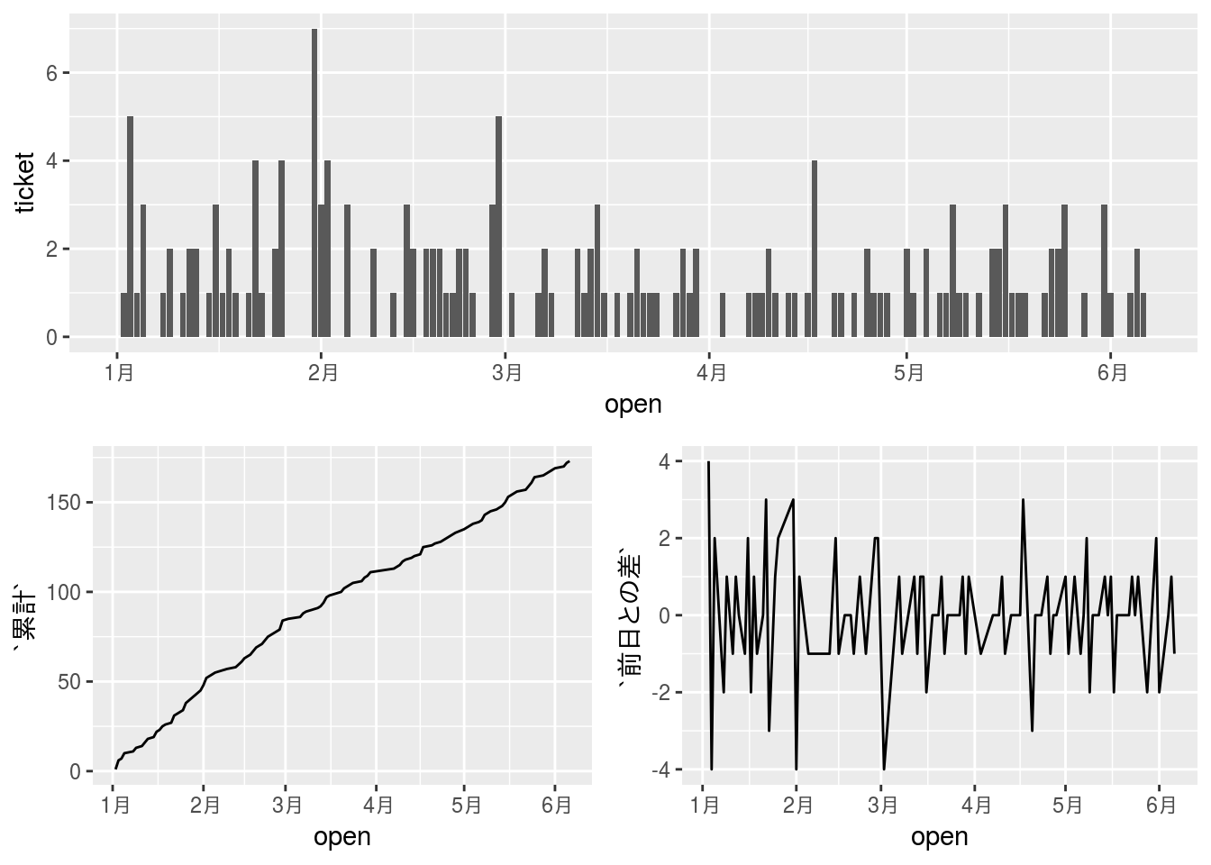
週次集計
“週”を求めるにはlubridate::week関数を用います。ただし、lubridate::week関数は1から53までの値しか返しませんので、年をまたぐ際はlubridate::year関数などを用いて年の識別ができるようにしてください。
なお、lubridate::week関数が返す週番号は1月1日を基準に単純に7日単位で計算した週番号です。ISOの週番号とは異なりますので注意してください。
起票されたチケットの推移
x %>%
  dplyr::filter(open >= "2018-1-1" & tracker == "Defect") %>%
  dplyr::mutate(week = lubridate::week(open)) %>%
  dplyr::filter(!is.na(week)) %>%
  dplyr::mutate(flag = ifelse(is.na(open), 0, 1)) %>%
  dplyr::group_by(week) %>%
  dplyr::summarise(ticket = sum(flag)) %>%
  dplyr::arrange(week) %>%
  dplyr::mutate(`累計` = cumsum(ticket),
`前週との差` = ticket - dplyr::lag(ticket))## # A tibble: 23 x 4
## week ticket 累計 前週との差
## <dbl> <dbl> <dbl> <dbl>
## 1 1 10 10 NA
## 2 2 8 18 -2
## 3 3 9 27 1
## 4 4 11 38 2
## 5 5 14 52 3
## 6 6 5 57 -9
## 7 7 10 67 5
## 8 8 9 76 -1
## 9 9 9 85 0
## 10 10 4 89 -5
## # ... with 13 more rowsgg_bar <- x %>%
dplyr::filter(open >= "2018-1-1" & tracker == "Defect") %>%
dplyr::mutate(week = lubridate::week(open)) %>%
dplyr::filter(!is.na(week)) %>%
dplyr::mutate(flag = ifelse(is.na(open), 0, 1)) %>%
dplyr::group_by(week) %>%
dplyr::summarise(ticket = sum(flag)) %>%
dplyr::arrange(week) %>%
dplyr::mutate(`累計` = cumsum(ticket),
`前週との差` = ticket - dplyr::lag(ticket)) %>%
ggplot2::ggplot(ggplot2::aes(x = week)) +
ggplot2::geom_bar(ggplot2::aes(y = ticket), stat = "identity")
gg_line <- x %>%
dplyr::filter(open >= "2018-1-1" & tracker == "Defect") %>%
dplyr::mutate(week = lubridate::week(open)) %>%
dplyr::filter(!is.na(week)) %>%
dplyr::mutate(flag = ifelse(is.na(open), 0, 1)) %>%
dplyr::group_by(week) %>%
dplyr::summarise(ticket = sum(flag)) %>%
dplyr::arrange(week) %>%
dplyr::mutate(`累計` = cumsum(ticket),
`前週との差` = ticket - dplyr::lag(ticket)) %>%
ggplot2::ggplot(ggplot2::aes(x = week)) +
ggplot2::geom_line(ggplot2::aes(y = `累計`))
gg_line_2 <- x %>%
dplyr::filter(open >= "2018-1-1" & tracker == "Defect") %>%
dplyr::mutate(week = lubridate::week(open)) %>%
dplyr::filter(!is.na(week)) %>%
dplyr::mutate(flag = ifelse(is.na(open), 0, 1)) %>%
dplyr::group_by(week) %>%
dplyr::summarise(ticket = sum(flag)) %>%
dplyr::arrange(week) %>%
dplyr::mutate(`累計` = cumsum(ticket),
`前週との差` = ticket - dplyr::lag(ticket)) %>%
ggplot2::ggplot(ggplot2::aes(x = week)) +
ggplot2::geom_line(ggplot2::aes(y = `前週との差`))
layout <- rbind(c(1, 1), c(2, 3))
gridExtra::grid.arrange(gg_bar, gg_line, gg_line_2, layout_matrix = layout)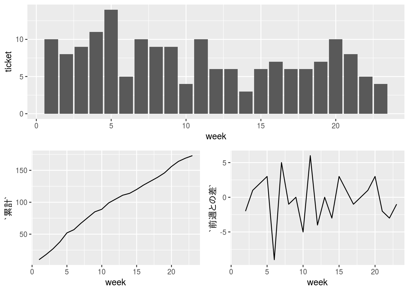
完了したチケットの推移
x %>%
  dplyr::filter(open >= "2018-1-1" & tracker == "Defect") %>%
  dplyr::mutate(week = lubridate::week(close)) %>%
  dplyr::filter(!is.na(week)) %>%
  dplyr::mutate(flag = ifelse(is.na(close), 0, 1)) %>%
  dplyr::group_by(week) %>%
  dplyr::summarise(ticket = sum(flag)) %>%
  dplyr::arrange(week) %>%
  dplyr::mutate(`累計` = cumsum(ticket),
`前週との差` = ticket - dplyr::lag(ticket))## # A tibble: 23 x 4
## week ticket 累計 前週との差
## <dbl> <dbl> <dbl> <dbl>
## 1 1 5 5 NA
## 2 2 3 8 -2
## 3 3 4 12 1
## 4 4 7 19 3
## 5 5 6 25 -1
## 6 6 2 27 -4
## 7 7 3 30 1
## 8 8 8 38 5
## 9 9 4 42 -4
## 10 10 2 44 -2
## # ... with 13 more rowsgg_bar <- x %>%
dplyr::filter(open >= "2018-1-1" & tracker == "Defect") %>%
dplyr::mutate(week = lubridate::week(close)) %>%
dplyr::filter(!is.na(week)) %>%
dplyr::mutate(flag = ifelse(is.na(close), 0, 1)) %>%
dplyr::group_by(week) %>%
dplyr::summarise(ticket = sum(flag)) %>%
dplyr::arrange(week) %>%
dplyr::mutate(`累計` = cumsum(ticket),
`前週との差` = ticket - dplyr::lag(ticket)) %>%
ggplot2::ggplot(ggplot2::aes(x = week)) +
ggplot2::geom_bar(ggplot2::aes(y = ticket), stat = "identity")
gg_line <- x %>%
dplyr::filter(open >= "2018-1-1" & tracker == "Defect") %>%
dplyr::mutate(week = lubridate::week(close)) %>%
dplyr::filter(!is.na(week)) %>%
dplyr::mutate(flag = ifelse(is.na(close), 0, 1)) %>%
dplyr::group_by(week) %>%
dplyr::summarise(ticket = sum(flag)) %>%
dplyr::arrange(week) %>%
dplyr::mutate(`累計` = cumsum(ticket),
`前週との差` = ticket - dplyr::lag(ticket)) %>%
ggplot2::ggplot(ggplot2::aes(x = week)) +
ggplot2::geom_line(ggplot2::aes(y = `累計`))
gg_line_2 <- x %>%
dplyr::filter(open >= "2018-1-1" & tracker == "Defect") %>%
dplyr::mutate(week = lubridate::week(close)) %>%
dplyr::filter(!is.na(week)) %>%
dplyr::mutate(flag = ifelse(is.na(close), 0, 1)) %>%
dplyr::group_by(week) %>%
dplyr::summarise(ticket = sum(flag)) %>%
dplyr::arrange(week) %>%
dplyr::mutate(`累計` = cumsum(ticket),
`前週との差` = ticket - dplyr::lag(ticket)) %>%
ggplot2::ggplot(ggplot2::aes(x = week)) +
ggplot2::geom_line(ggplot2::aes(y = `前週との差`))
layout <- rbind(c(1, 1), c(2, 3))
gridExtra::grid.arrange(gg_bar, gg_line, gg_line_2, layout_matrix = layout)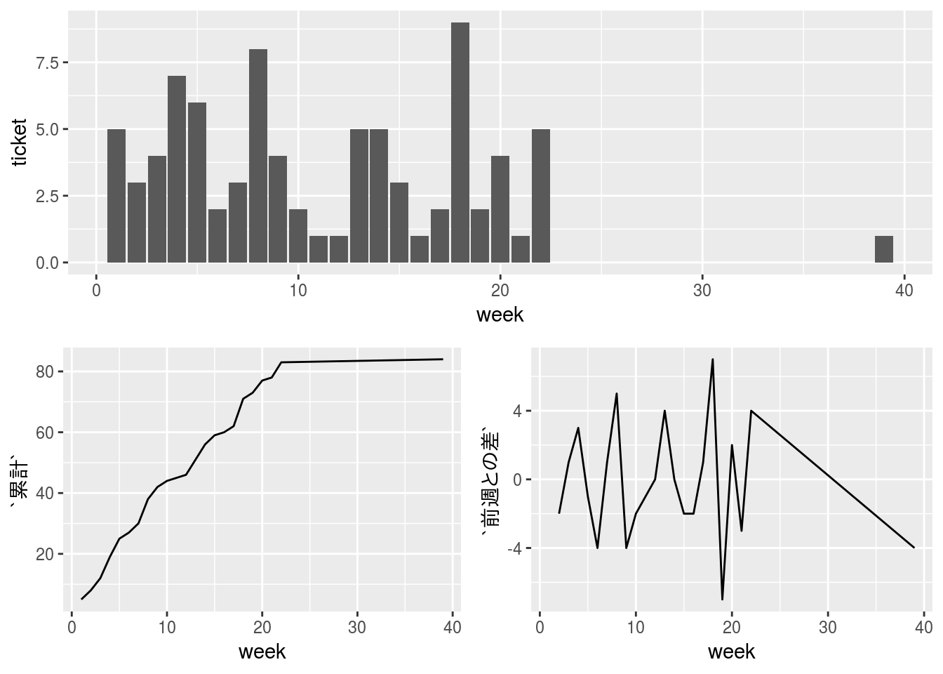
月次集計
“月”を求めるにはlubridate::month関数を用います。ただし、lubridate::month関数は1から12までの値しか返しませんので、年をまたぐ際はlubridate::year関数などを用いて年の識別ができるようにしてください。
起票されたチケットの推移
x %>%
  dplyr::filter(open >= "2018-1-1" & tracker == "Defect") %>%
  dplyr::mutate(month = lubridate::month(open)) %>%
  dplyr::mutate(flag = ifelse(is.na(open), 0, 1)) %>%
  dplyr::group_by(month) %>%
  dplyr::summarise(ticket = sum(flag)) %>%
  dplyr::arrange(month) %>%
  dplyr::mutate(`累計` = cumsum(ticket),
`前月との差` = ticket - dplyr::lag(ticket))## # A tibble: 6 x 4
## month ticket 累計 前月との差
## <dbl> <dbl> <dbl> <dbl>
## 1 1 45 45 NA
## 2 2 39 84 -6
## 3 3 27 111 -12
## 4 4 22 133 -5
## 5 5 35 168 13
## 6 6 5 173 -30gg_bar <- x %>%
dplyr::filter(open >= "2018-1-1" & tracker == "Defect") %>%
dplyr::mutate(month = lubridate::month(open)) %>%
dplyr::mutate(flag = ifelse(is.na(open), 0, 1)) %>%
dplyr::group_by(month) %>%
dplyr::summarise(ticket = sum(flag)) %>%
dplyr::arrange(month) %>%
dplyr::mutate(`累計` = cumsum(ticket),
`前月との差` = ticket - dplyr::lag(ticket)) %>%
ggplot2::ggplot(ggplot2::aes(x = month)) +
ggplot2::geom_bar(ggplot2::aes(y = ticket), stat = "identity")
gg_line <- x %>%
dplyr::filter(open >= "2018-1-1" & tracker == "Defect") %>%
dplyr::mutate(month = lubridate::month(open)) %>%
dplyr::mutate(flag = ifelse(is.na(open), 0, 1)) %>%
dplyr::group_by(month) %>%
dplyr::summarise(ticket = sum(flag)) %>%
dplyr::arrange(month) %>%
dplyr::mutate(`累計` = cumsum(ticket),
`前月との差` = ticket - dplyr::lag(ticket)) %>%
ggplot2::ggplot(ggplot2::aes(x = month)) +
ggplot2::geom_line(ggplot2::aes(y = `累計`))
gg_line_2 <- x %>%
dplyr::filter(open >= "2018-1-1" & tracker == "Defect") %>%
dplyr::mutate(month = lubridate::month(open)) %>%
dplyr::mutate(flag = ifelse(is.na(open), 0, 1)) %>%
dplyr::group_by(month) %>%
dplyr::summarise(ticket = sum(flag)) %>%
dplyr::arrange(month) %>%
dplyr::mutate(`累計` = cumsum(ticket),
`前月との差` = ticket - dplyr::lag(ticket)) %>%
ggplot2::ggplot(ggplot2::aes(x = month)) +
ggplot2::geom_line(ggplot2::aes(y = `前月との差`))
layout <- rbind(c(1, 1), c(2, 3))
gridExtra::grid.arrange(gg_bar, gg_line, gg_line_2, layout_matrix = layout)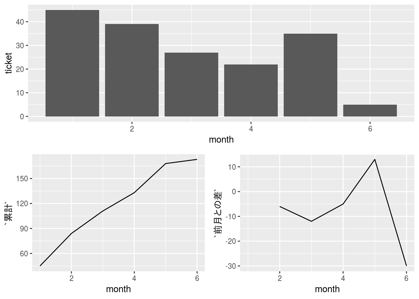
四半期次集計
“四半期”を求めるにはlubridate::quarter関数を用います。年をまたぐ際はwith_yearオプションを使用すると年の識別ができるようになります。また、第一四半期が1月以外から始まる場合はfiscal_startオプションを使用してください。
起票されたチケットの推移
x %>%
  dplyr::filter(tracker == "Defect") %>%
  dplyr::mutate(quarter = lubridate::quarter(open, with_year = TRUE,
                                             fiscal_start = 1)) %>%
  dplyr::mutate(flag = ifelse(is.na(open), 0, 1)) %>%
  dplyr::group_by(quarter) %>%
  dplyr::summarise(ticket = sum(flag)) %>%
  dplyr::arrange(quarter) %>%
  dplyr::mutate(`累計` = cumsum(ticket),
`前四半期との差` = ticket - dplyr::lag(ticket))## # A tibble: 21 x 4
## quarter ticket 累計 前四半期との差
## <dbl> <dbl> <dbl> <dbl>
## 1 2013. 188 188 NA
## 2 2013. 207 395 19
## 3 2013. 161 556 -46
## 4 2014. 174 730 13
## 5 2014. 136 866 -38
## 6 2014. 136 1002 0
## 7 2014. 131 1133 -5
## 8 2015. 236 1369 105
## 9 2015. 143 1512 -93
## 10 2015. 146 1658 3
## # ... with 11 more rows
lubridate::quarter関数の返り値はnumeric型ですので棒グラフにする場合は文字列型または因子型に変換する必要がある点に注意してください。
x %>%
  dplyr::filter(tracker == "Defect") %>%
  dplyr::mutate(quarter = lubridate::quarter(open, with_year = TRUE,
                                             fiscal_start = 1)) %>%
  dplyr::mutate(flag = ifelse(is.na(open), 0, 1)) %>%
  dplyr::group_by(quarter) %>%
  dplyr::summarise(ticket = sum(flag)) %>%
  dplyr::arrange(quarter) %>%
  dplyr::mutate(quarter = as.character(quarter),
                `累計` = cumsum(ticket),
                `前四半期との差` = ticket - dplyr::lag(ticket)) %>%
  ggplot2::ggplot(ggplot2::aes(x = quarter)) +
    ggplot2::geom_bar(ggplot2::aes(y = ticket), stat = "identity")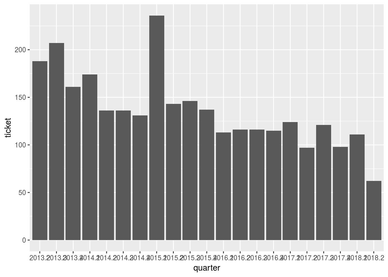
同様に折れ線グラフにする場合にもquarterの扱いには注意が必要です。
# x_name <- x %>%
#   dplyr::filter(tracker == "Defect") %>%
#   dplyr::mutate(quarter = lubridate::quarter(open, with_year = TRUE,
#                                              fiscal_start = 1)) %>%
#   dplyr::mutate(quarter = as.character(quarter)) %>%
#   dplyr::distinct(quarter) %>%
#   dplyr::arrange(quarter)

x %>%
  dplyr::filter(tracker == "Defect") %>%
  dplyr::mutate(quarter = lubridate::quarter(open, with_year = TRUE,
                                             fiscal_start = 1)) %>%
  dplyr::mutate(flag = ifelse(is.na(open), 0, 1)) %>%
  dplyr::group_by(quarter) %>%
  dplyr::summarise(ticket = sum(flag)) %>%
  dplyr::arrange(quarter) %>%
  dplyr::mutate(`累計` = cumsum(ticket),
`前四半期との差` = ticket - dplyr::lag(ticket))## # A tibble: 21 x 4
## quarter ticket 累計 前四半期との差
## <dbl> <dbl> <dbl> <dbl>
## 1 2013. 188 188 NA
## 2 2013. 207 395 19
## 3 2013. 161 556 -46
## 4 2014. 174 730 13
## 5 2014. 136 866 -38
## 6 2014. 136 1002 0
## 7 2014. 131 1133 -5
## 8 2015. 236 1369 105
## 9 2015. 143 1512 -93
## 10 2015. 146 1658 3
## # ... with 11 more rows
年次集計
“年”を求めるにはlubridate::year関数を用います。
起票されたチケットの推移
x %>%
  dplyr::filter(tracker == "Defect") %>%
  dplyr::mutate(year = lubridate::year(open)) %>%
  dplyr::mutate(flag = ifelse(is.na(open), 0, 1)) %>%
  dplyr::group_by(year) %>%
  dplyr::summarise(ticket = sum(flag)) %>%
  dplyr::arrange(year) %>%
  dplyr::mutate(`累計` = cumsum(ticket),
`前年との差` = ticket - dplyr::lag(ticket))## # A tibble: 6 x 4
## year ticket 累計 前年との差
## <dbl> <dbl> <dbl> <dbl>
## 1 2013 556 556 NA
## 2 2014 577 1133 21
## 3 2015 662 1795 85
## 4 2016 460 2255 -202
## 5 2017 440 2695 -20
## 6 2018 173 2868 -267gg_bar <- x %>%
dplyr::filter(tracker == "Defect") %>%
dplyr::mutate(year = lubridate::year(open)) %>%
dplyr::mutate(flag = ifelse(is.na(open), 0, 1)) %>%
dplyr::group_by(year) %>%
dplyr::summarise(ticket = sum(flag)) %>%
dplyr::arrange(year) %>%
dplyr::mutate(`累計` = cumsum(ticket),
`前年との差` = ticket - dplyr::lag(ticket)) %>%
ggplot2::ggplot(ggplot2::aes(x = year)) +
ggplot2::geom_bar(ggplot2::aes(y = ticket), stat = "identity")
gg_line <- x %>%
dplyr::filter(tracker == "Defect") %>%
dplyr::mutate(year = lubridate::year(open)) %>%
dplyr::mutate(flag = ifelse(is.na(open), 0, 1)) %>%
dplyr::group_by(year) %>%
dplyr::summarise(ticket = sum(flag)) %>%
dplyr::arrange(year) %>%
dplyr::mutate(`累計` = cumsum(ticket),
`前年との差` = ticket - dplyr::lag(ticket)) %>%
ggplot2::ggplot(ggplot2::aes(x = year)) +
ggplot2::geom_line(ggplot2::aes(y = `累計`))
gg_line_2 <- x %>%
dplyr::filter(tracker == "Defect") %>%
dplyr::mutate(year = lubridate::year(open)) %>%
dplyr::mutate(flag = ifelse(is.na(open), 0, 1)) %>%
dplyr::group_by(year) %>%
dplyr::summarise(ticket = sum(flag)) %>%
dplyr::arrange(year) %>%
dplyr::mutate(`累計` = cumsum(ticket),
`前年との差` = ticket - dplyr::lag(ticket)) %>%
ggplot2::ggplot(ggplot2::aes(x = year)) +
ggplot2::geom_line(ggplot2::aes(y = `前年との差`))
layout <- rbind(c(1, 1), c(2, 3))
gridExtra::grid.arrange(gg_bar, gg_line, gg_line_2, layout_matrix = layout)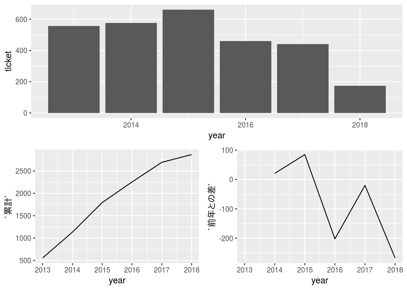
グラフによる可視化
可視化にグラフを用いると変化や差異が把握しやすくなりますので分析の目的にあったグラフを持ちいることが大切です。
分布の可視化
分布を可視化する代表的な方法としてはヒストグラム、箱ひげ図などがあります。
滞留期間の可視化
2018年のチケットが優先度ごとにどれだけ期間滞留しているかを可視化してみます。分布を把握したい場合はヒストグラム、分布範囲を把握した場合は箱ひげ図が便利です。
x %>%
  dplyr::filter(open >= "2018-1-1" & tracker == "Defect") %>%
  dplyr::filter(status != "Closed") %>%
  dplyr::mutate(days = lubridate::today() - open + 1) %>%
  dplyr::group_by(priority) %>%
dplyr::summarise(min = min(days), med = median(days), max = max(days))## # A tibble: 4 x 4
## priority min med max
## <ord> <time> <time> <time>
## 1 Low 241 days 274.0 days 307 days
## 2 Normal 158 days 239.5 days 312 days
## 3 High 170 days 241.0 days 297 days
## 4 Urgent 249 days 259.5 days 270 daysgg_bar <- x %>%
dplyr::filter(open >= "2018-1-1" & tracker == "Defect") %>%
dplyr::filter(status != "Closed") %>%
dplyr::mutate(days = lubridate::today() - open + 1) %>%
ggplot2::ggplot(ggplot2::aes(x = days, fill = priority)) +
ggplot2::geom_histogram(alpha = 0.5, position = "identity")
gg_boxplot <- x %>%
dplyr::filter(open >= "2018-1-1" & tracker == "Defect") %>%
dplyr::filter(status != "Closed") %>%
dplyr::mutate(days = lubridate::today() - open + 1) %>%
ggplot2::ggplot(ggplot2::aes(x = priority, y = days, colour = priority)) +
ggplot2::geom_boxplot() +
ggplot2::geom_jitter() +
ggplot2::coord_flip()
gridExtra::grid.arrange(gg_bar, gg_boxplot, nrow = 2)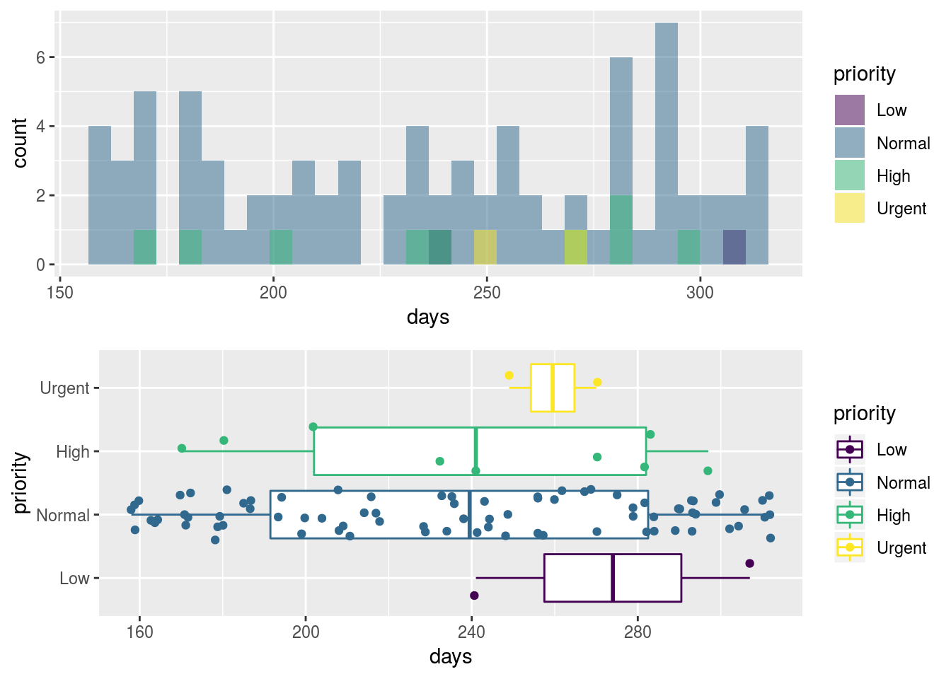
同様にカテゴリごとの滞留期間を可視化してみます。
x %>%
  dplyr::filter(open >= "2018-1-1") %>%
  dplyr::filter(status != "Closed") %>%
  dplyr::mutate(days = lubridate::today() - open + 1) %>%
  dplyr::group_by(category) %>%
  dplyr::summarise(min = min(days), med = median(days), max = max(days),
mode = which.max(table(days)))## # A tibble: 34 x 5
## category min med max mode
## <chr> <time> <time> <time> <int>
## 1 Accounts / authentication 170 days 211 days 270 days 1
## 2 Activity view 243 days 243 days 243 days 1
## 3 Administration 164 days 217 days 270 days 1
## 4 Attachments 229 days 229 days 229 days 1
## 5 Calendar 201 days 201 days 201 days 1
## 6 Code cleanup/refactoring 163 days 218 days 294 days 1
## 7 Custom fields 164 days 172 days 293 days 2
## 8 Database 232 days 232 days 232 days 1
## 9 Documentation 160 days 241 days 249 days 1
## 10 Email receiving 171 days 234 days 312 days 1
## # ... with 24 more rowsx %>%
dplyr::filter(open >= "2018-1-1") %>%
dplyr::filter(status != "Closed") %>%
dplyr::mutate(days = lubridate::today() - open + 1) %>%
ggplot2::ggplot(ggplot2::aes(x = category, y = days)) +
ggplot2::geom_boxplot()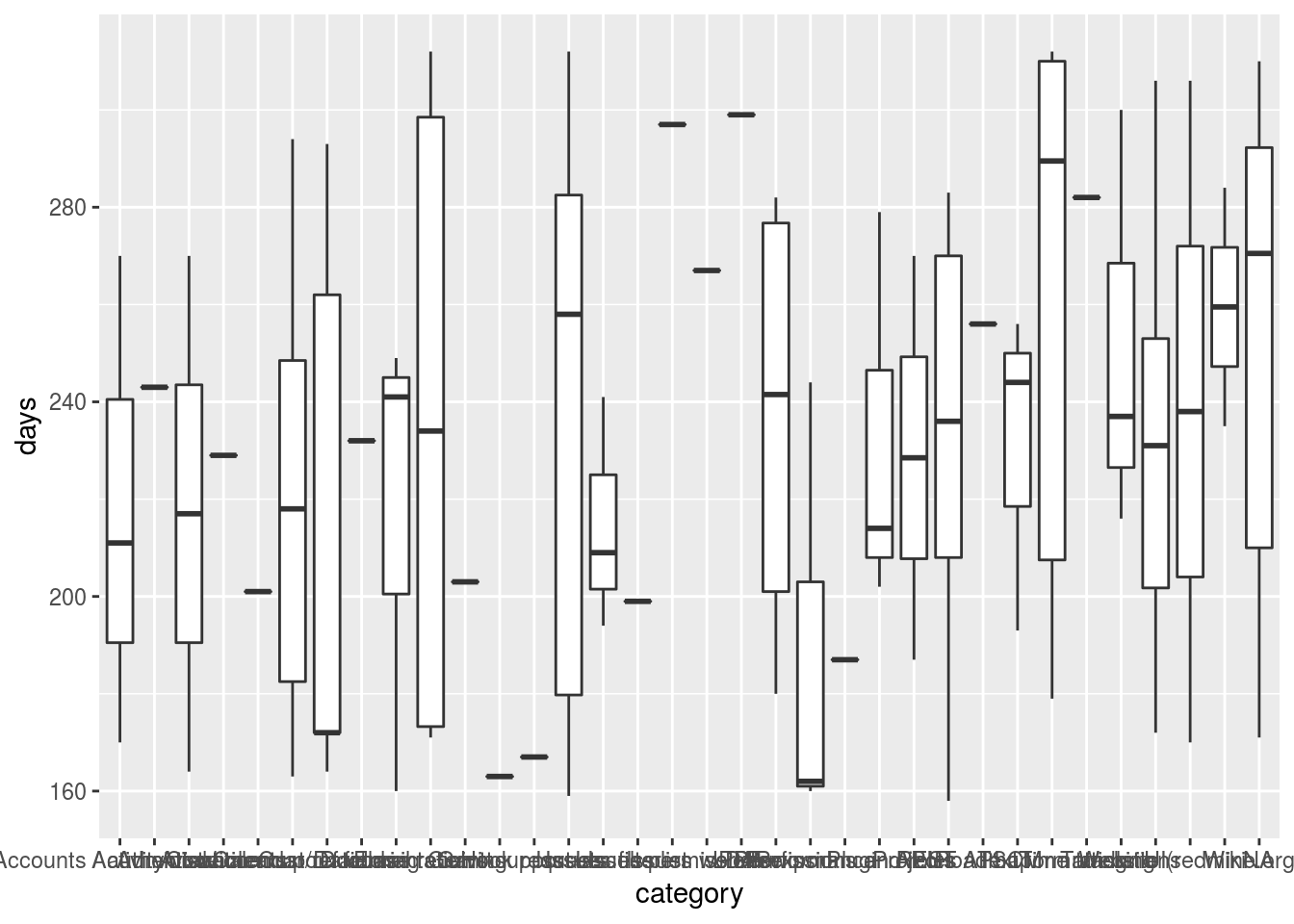
対処期間の可視化
カテゴリごとのチケット対処期間(開始日から終了日までの期間)を可視化してみます。
x %>%
  dplyr::filter(status == "Closed") %>%
  dplyr::mutate(days = close - open + 1) %>%
  dplyr::group_by(category) %>%
  dplyr::summarise(min = min(days), med = median(days), max = max(days),
mode = which.max(table(days)))## # A tibble: 56 x 5
## category min med max mode
## <chr> <time> <time> <time> <int>
## 1 Accounts / authentication 1 days " 3.5 days" 1369 days 1
## 2 Activity view 1 days " 6.0 days" 1247 days 1
## 3 Administration 1 days " 2.0 days" " 167 days" 1
## 4 Attachments 1 days 10.0 days " 814 days" 2
## 5 Calendar 1 days 51.0 days " 386 days" 1
## 6 Code cleanup/refactoring 1 days " 8.0 days" " 499 days" 1
## 7 Core Plugins 2 days " 2.0 days" " 6 days" 1
## 8 Custom fields 1 days 11.0 days 1211 days 1
## 9 Database 1 days " 2.0 days" 1195 days 1
## 10 Documentation 1 days " 2.0 days" " 668 days" 1
## # ... with 46 more rowsx %>%
dplyr::filter(status == "Closed") %>%
dplyr::mutate(days = close - open + 1) %>%
ggplot2::ggplot(ggplot2::aes(x = category, y = days)) +
ggplot2::geom_boxplot()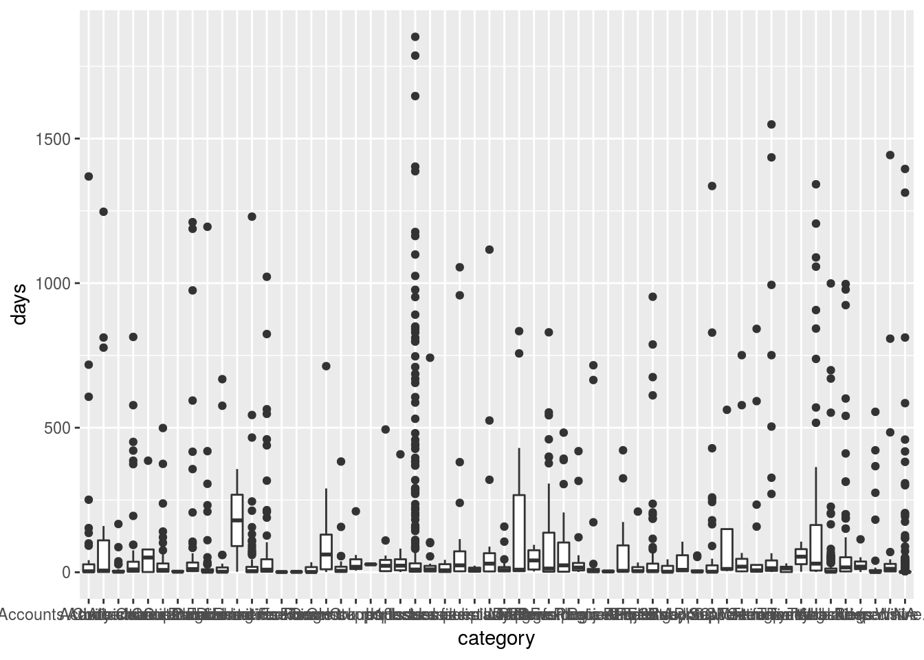
比率の可視化
集計結果の比率(割合)を可視化する方法としては棒グラフ、円グラフ、およびそれらの層別グラフなどがあります。層別するメリットは因子の水準ごとの違いの有無が把握できるようになることです。
Priority vs Category, Open Tickets
x %>%
  dplyr::filter(status != "Closed" & tracker == "Defect") %>%
  dplyr::mutate(year = lubridate::year(open)) %>%
  ggplot2::ggplot(ggplot2::aes(x = priority, fill = category)) +
    ggplot2::geom_bar(alpha = 0.5) +
    ggplot2::facet_wrap(~ year)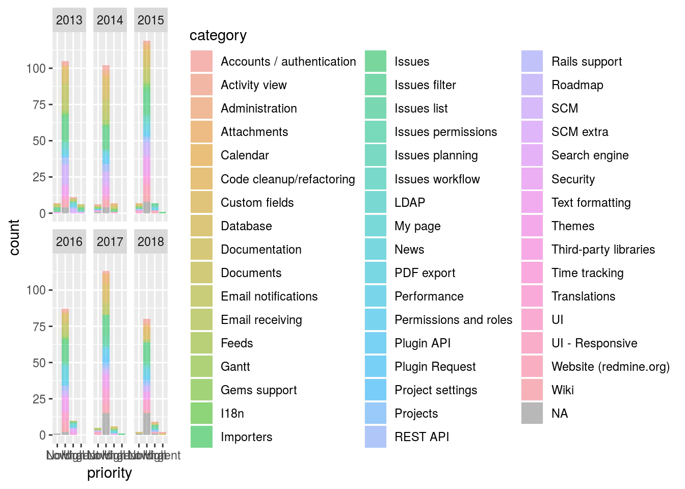
Priority vs Category, Closed Tickets
x %>%
  dplyr::filter(status == "Closed" & tracker == "Defect") %>%
  dplyr::mutate(year = lubridate::year(close)) %>%
  ggplot2::ggplot(ggplot2::aes(x = priority, fill = category)) +
    ggplot2::geom_bar(alpha = 0.5) +
    ggplot2::facet_wrap(~ year)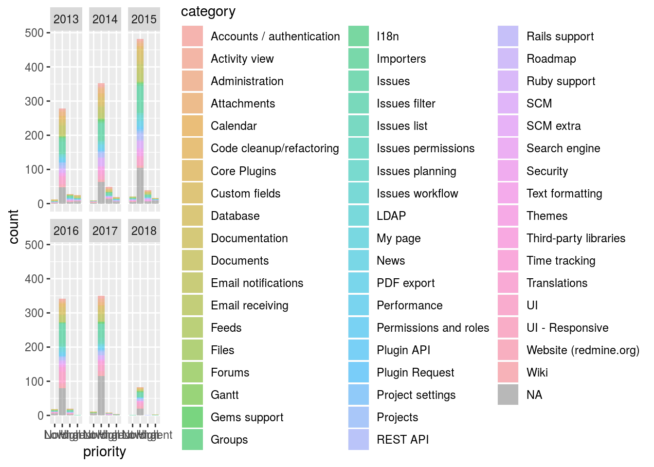
Affected version vs Status
比率の可視化に利用する棒グラフも時系列で層別に描くと推移もみえるようになります。例えば、バージョンごとのチケットの完了状況をチケット起票年ごとに分けて表示することで過去バグと最近のバグの発生状況が俯瞰できるようになります。
x %>%
  dplyr::filter(tracker == "Defect") %>%
  dplyr::mutate(flag = ifelse(status == "Closed", "Closed", "Open")) %>%
  dplyr::mutate(year = lubridate::year(open)) %>%
  dplyr::filter(!is.na(affected)) %>%
  ggplot2::ggplot(ggplot2::aes(x = affected, fill = flag)) +
    ggplot2::geom_bar(alpha = 0.75) +
    ggplot2::facet_wrap(~ year)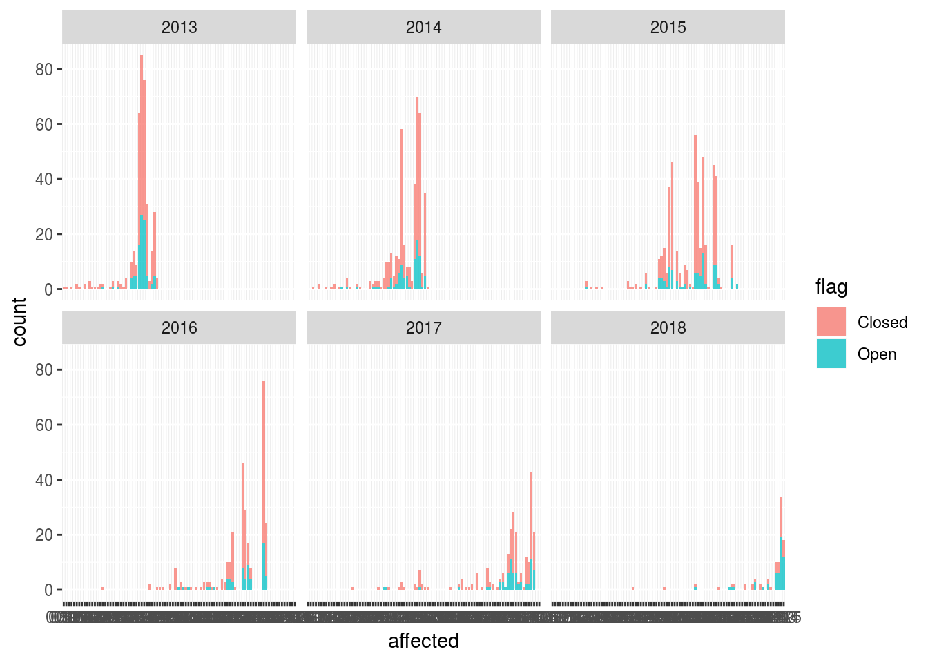
推移の可視化
(主に時系列の)推移を可視化する代表的な方法としては折れ線グラフ、棒グラフ、ヒートマップがあります。
四半期ごとの完了チケット数
棒グラフを用いると時系列による比率の変化がみえるようになります。
x %>%
  dplyr::filter(tracker == "Defect") %>%
  dplyr::mutate(quarter = lubridate::quarter(close, with_year = TRUE,
                                             fiscal_start = 1)) %>%
  dplyr::mutate(flag = ifelse(is.na(close), 0, 1)) %>%
  dplyr::group_by(quarter, priority) %>%
  dplyr::summarise(ticket = sum(flag)) %>%
  dplyr::arrange(quarter) %>%
  dplyr::filter(!is.na(quarter)) %>%
  dplyr::mutate(`累計` = cumsum(ticket),
                `前四半期との差` = ticket - dplyr::lag(ticket)) %>%
  ggplot2::ggplot(ggplot2::aes(x = as.character(quarter))) +
    ggplot2::geom_bar(ggplot2::aes(y = ticket, fill = priority),
                      stat = "identity", alpha = 0.5) +
    ggplot2::labs(x = "", y = "Number of 'Closed' Defect Ticket",
                  title = "四半期ごとの完了バグチケット数の推移")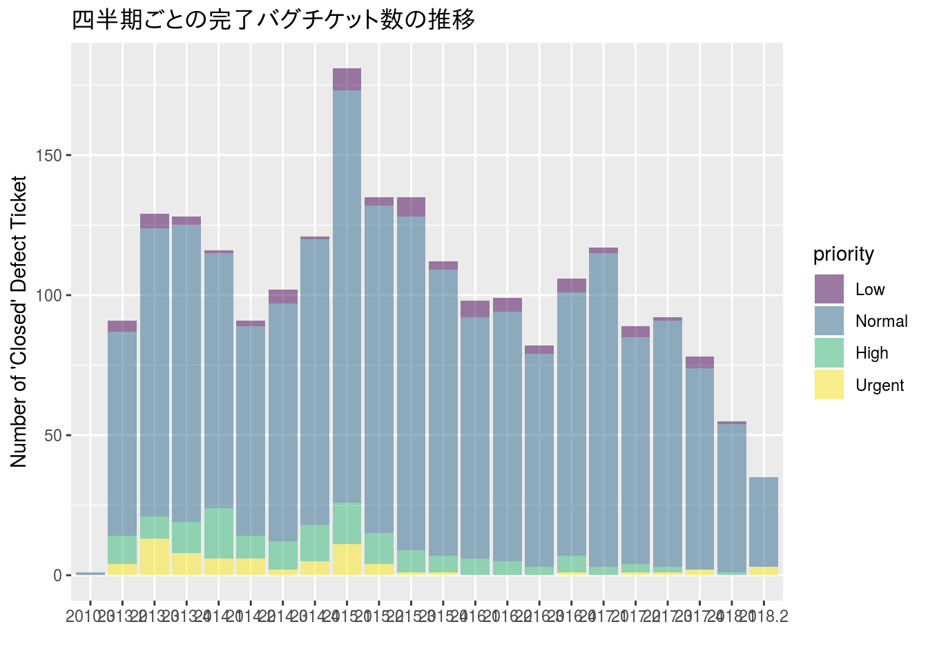
週次傾向の可視化
前出の週次集計を可視化してみます。加えて平均起票数を基準として前週との起票数の差を折れ線グラフで表示しています。
open <- x %>%
  dplyr::filter(open >= "2018-1-1" & tracker == "Defect") %>%
  dplyr::mutate(week = lubridate::week(open)) %>%
  dplyr::filter(!is.na(week))

close <- x %>%
  dplyr::filter(open >= "2018-1-1" & tracker == "Defect") %>%
  dplyr::filter(close >= "2018-1-1") %>%
  dplyr::mutate(week = lubridate::week(close)) %>%
  dplyr::filter(!is.na(week))

df_week <-
  seq(ifelse(min(open$week) <= min(close$week), min(open$week), min(close$week)),
      ifelse(max(open$week) >= max(close$week), max(open$week), max(close$week)),
      by = 1) %>% as.data.frame()
names(df_week) <- c("week")
起票されたチケットの推移
open <- x %>%
  dplyr::filter(open >= "2018-1-1" & tracker == "Defect") %>%
  dplyr::mutate(week = lubridate::week(open)) %>%
  dplyr::filter(!is.na(week))

open <- df_week %>%
  dplyr::left_join(open, by = "week") %>%
  dplyr::mutate(flag = ifelse(is.na(open), 0, 1)) %>%
  dplyr::group_by(week) %>%
  dplyr::summarise(open = sum(flag)) %>%
  dplyr::arrange(week) %>%
  dplyr::mutate(cumopen = cumsum(open), diff = open - dplyr::lag(open))

open %>%
  dplyr::rename(`週` = week, `チケットオープン数` = open, `累計` = cumopen,
`前週との差` = diff)## # A tibble: 23 x 4
## 週 チケットオープン数 累計 前週との差
## <dbl> <dbl> <dbl> <dbl>
## 1 1 10 10 NA
## 2 2 8 18 -2
## 3 3 9 27 1
## 4 4 11 38 2
## 5 5 14 52 3
## 6 6 5 57 -9
## 7 7 10 67 5
## 8 8 9 76 -1
## 9 9 9 85 0
## 10 10 4 89 -5
## # ... with 13 more rowsopen %>%
dplyr::mutate(diff_offset = diff + round(mean(open, na.rm = TRUE))) %>%
ggplot2::ggplot(ggplot2::aes(x = week)) +
ggplot2::geom_bar(ggplot2::aes(y = open), stat = "identity", alpha = 0.25) +
ggplot2::geom_hline(yintercept = round(mean(open$open, na.rm = TRUE), 1),
colour = "#00bfc4", linetype = "dashed") +
ggplot2::geom_line(ggplot2::aes(y = diff_offset), colour = "#00bfc4",
size = 0.75)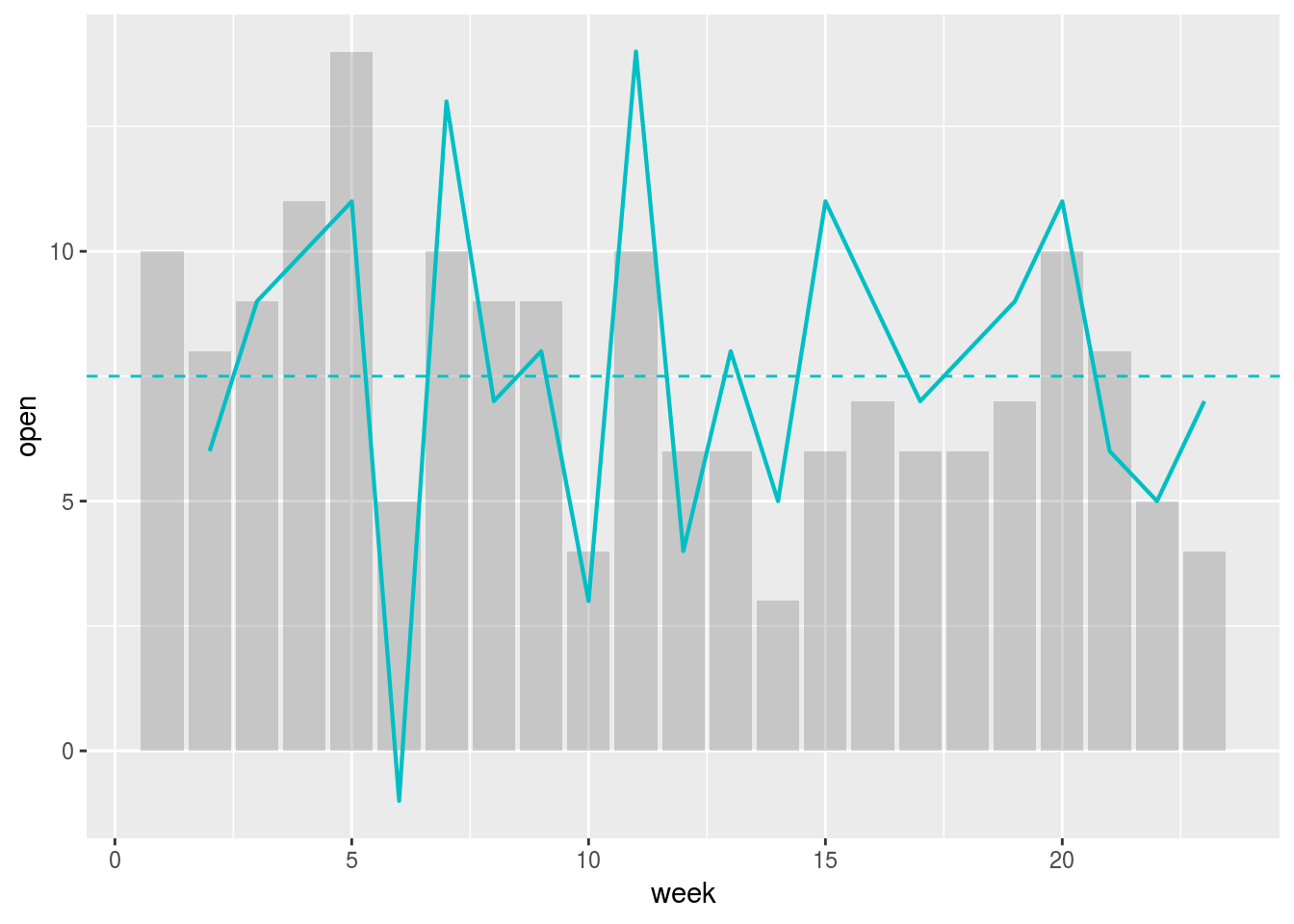
ここではチケット数のみグラフにしていますが、試験実施数を試験種別などで色分けした棒グラフなどを重ね合わせることで実施に対してどれだけのバグが摘出できているかがみえてくるようになる可能性があります。
完了したチケットの推移
同様に対処が完了したチケット数をグラフにしてみます。
close <- x %>%
  dplyr::filter(open >= "2018-1-1" & tracker == "Defect") %>%
  dplyr::filter(close >= "2018-1-1") %>%
  dplyr::mutate(week = lubridate::week(close)) %>%
  dplyr::filter(!is.na(week))

close <- df_week %>%
  dplyr::left_join(close, by = "week") %>%
  dplyr::mutate(flag = ifelse(is.na(close), 0, 1)) %>%
  dplyr::group_by(week) %>%
  dplyr::summarise(close = sum(flag)) %>%
  dplyr::arrange(week) %>%
  dplyr::mutate(cumclose = cumsum(close), diff = close -dplyr::lag(close))

close %>%
  dplyr::rename(`週` = week, `チケットクローズ数` = close, `累計` = cumclose,
`前週との差` = diff)## # A tibble: 23 x 4
## 週 チケットクローズ数 累計 前週との差
## <dbl> <dbl> <dbl> <dbl>
## 1 1 5 5 NA
## 2 2 3 8 -2
## 3 3 4 12 1
## 4 4 7 19 3
## 5 5 6 25 -1
## 6 6 2 27 -4
## 7 7 3 30 1
## 8 8 8 38 5
## 9 9 4 42 -4
## 10 10 2 44 -2
## # ... with 13 more rowsclose %>%
dplyr::mutate(diff_offset = diff + round(mean(close, na.rm = TRUE)), 1) %>%
ggplot2::ggplot(ggplot2::aes(x = week)) +
ggplot2::geom_bar(ggplot2::aes(y = close), stat = "identity", alpha = 0.25) +
ggplot2::geom_hline(yintercept = round(mean(close$close, na.rm = TRUE)),
colour = "#f8766d", linetype = "dashed") +
ggplot2::geom_line(ggplot2::aes(y = diff_offset), colour = "#f8766d",
size = 0.75)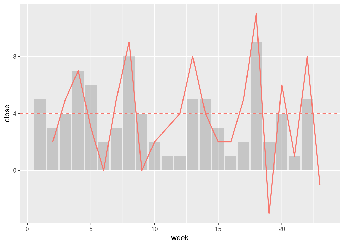
チケットのオープン数と比べるとクローズ数の方がかなり低調に見えます。
オープン・クローズチャート
前出の週次の集計から累計データに着目したものがオープン・クローズチャートです。オープン・クローズチャートはチケットの対応状況が一目で分かるグラフです。
week_ticket <- open %>%
  dplyr::full_join(close, by = "week") %>%
  dplyr::select(week, open, close) %>%
  tidyr::gather(key, value, -week)

open %>%
  dplyr::full_join(close, by = "week") %>%
  dplyr::select(week, cumopen, cumclose) %>%
  tidyr::gather(key, value, -week) %>%
  dplyr::left_join(week_ticket, by = "week") %>%
  ggplot2::ggplot(ggplot2::aes(x = week)) +
    ggplot2::geom_bar(ggplot2::aes(y = value.y, fill = key.y),
                      stat = "identity", alpha = 0.5, position = "dodge") +
    ggplot2::geom_line(ggplot2::aes(y = value.x, colour = key.x),
                       stat = "identity", size = 0.75) +
    ggplot2::scale_color_hue(name = "累計",
                             labels = c(cumclose = "Closed", cumopen = "Open")) +
    ggplot2::scale_fill_hue(name = "週次",
                            labels = c(close = "Closed", open = "Open")) +
    ggplot2::labs(y = "Number of Defect Ticket",
                  title = "週次のバグチケット数の推移")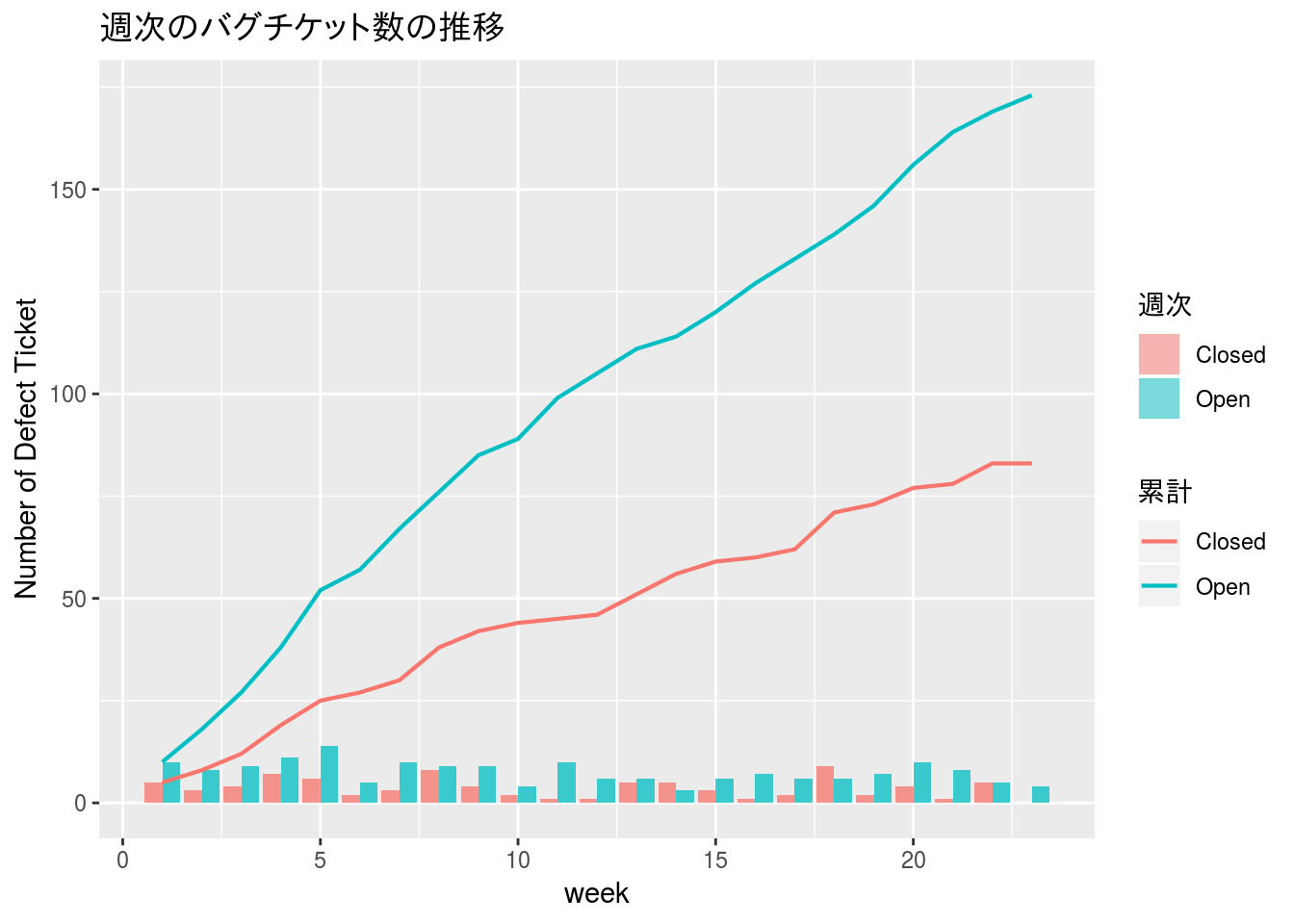
個別にチャートを描いた場合に見えたようにクローズ傾向が低調なため処理が完了しないチケットが増えていることが分かります。
このグラフに試験項目数(計画、実績)のバーンダウンチャートを加えれば週次管理表になります。
日次のオープン・クローズチャート
日次の場合は試験稼働が発生していない日はチケット起票がゼロとは言えず、無稼働日を除かないとチャートが横に寝てしまい正しい傾向が掴めませんので注意してください。
open <- x %>%
  dplyr::filter(open >= "2018-1-1" & tracker == "Defect") %>%
  dplyr::filter(!is.na(open))

close <- x %>%
  dplyr::filter(open >= "2018-1-1" & tracker == "Defect") %>%
  dplyr::filter(close >= "2018-1-1") %>%
  dplyr::filter(!is.na(close))

start <- ifelse(range(open$open)[1] <= range(close$close)[1],
                range(open$open)[1], range(close$close)[1]) %>%
  lubridate::as_date()

end <- ifelse(range(open$open)[2] <= range(close$close)[2],
              range(open$open)[2], range(close$close)[2]) %>%
  lubridate::as_date()

df_days <-
  seq(start, end, by = 1) %>% as.data.frame()
names(df_days) <- c("days")

open_ticket <- df_days %>%
  dplyr::left_join(open, by = c("days" = "open")) %>%
  dplyr::mutate(flag = ifelse(is.na(no), 0, 1)) %>%
  dplyr::group_by(days) %>%
  dplyr::summarise(open = sum(flag)) %>%
  dplyr::arrange(days) %>%
  dplyr::mutate(cumopen = cumsum(open))

close_ticket <- df_days %>%
  dplyr::left_join(close, by = c("days" = "close")) %>%
  dplyr::mutate(flag = ifelse(is.na(no), 0, 1)) %>%
  dplyr::group_by(days) %>%
  dplyr::summarise(close = sum(flag)) %>%
  dplyr::arrange(days) %>%
  dplyr::mutate(cumclose = cumsum(close))

bar_data <- open_ticket %>%
  dplyr::left_join(close_ticket, by = "days") %>%
  dplyr::select(days, open, close) %>%
  tidyr::gather(key, value , -days)

line_data <- open_ticket %>%
  dplyr::left_join(close_ticket, by = "days") %>%
  dplyr::select(days, cumopen, cumclose) %>%
  tidyr::gather(key, value , -days)

bar_data %>%
  dplyr::left_join(line_data, by = "days") %>%
  ggplot2::ggplot(ggplot2::aes(x = days)) +
    ggplot2::geom_bar(ggplot2::aes(y = value.x, fill = key.x),
                      stat = "identity", alpha = 0.5, position = "dodge") +
    ggplot2::geom_line(ggplot2::aes(y = value.y, colour = key.y),
                       stat = "identity", size = 0.75) +
    ggplot2::scale_color_hue(name = "累計",
                             labels = c(cumclose = "Closed", cumopen = "Open")) +
    ggplot2::scale_fill_hue(name = "日次",
                            labels = c(close = "Closed", open = "Open")) +
    ggplot2::labs(y = "Number of Defect Ticket",
                  title = "日次のバグチケット数の推移")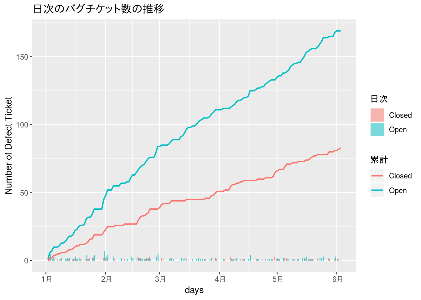
ヒートマップ
推移を見るには前述のように折れ線グラフや棒グラフを利用することが多いですが、対象期間が長くなるとグラフが見難くなる場合があります。そんな時に便利なグラフがヒートマップです。数値の大小を色で表で表しますので、特にピークやボトムの推移を把握するのに向いています。
x %>%
  dplyr::filter(tracker == "Defect") %>%
  dplyr::select(date = open) %>%
  dplyr::count(date) %>%
# ヒートマップに項目に応じて年、月、週、日、曜日などを求める
  dplyr::mutate(year = lubridate::year(date), month = lubridate::month(date),
                week = lubridate::epiweek(date), day = lubridate::day(date),
                wday = lubridate::wday(date, label = TRUE, week_start = 7),
                tweek = lubridate::epiweek(lubridate::floor_date(date, "month"))) %>%
# 特有の処理
  dplyr::mutate(offset = ifelse(tweek == 53, 54, 1)) %>%
  dplyr::mutate(offset = ifelse(tweek == 52, 53, offset)) %>%
  dplyr::mutate(offset = ifelse(tweek > week, tweek - week + 1, offset)) %>%
# 例外処理
  dplyr::mutate(offset = ifelse(tweek == week, 1, offset)) %>%
# 月内の週数を計算する
  dplyr::mutate(mweek = week - tweek + offset) %>%
  # dplyr::filter(year == 2016) %>%
  # dplyr::mutate(mweek = mweek(date)) %>%      # ベクトル対応できていない
  # print()
  ggplot2::ggplot(ggplot2::aes(x = wday, y = mweek, fill = n)) +
    ggplot2::facet_grid(year ~ month) +
    ggplot2::geom_tile() +
    ggplot2::scale_fill_gradient(low = "lightyellow", high = "red") +
    ggplot2::labs(x = "", y = "") +
    ggplot2::theme_bw()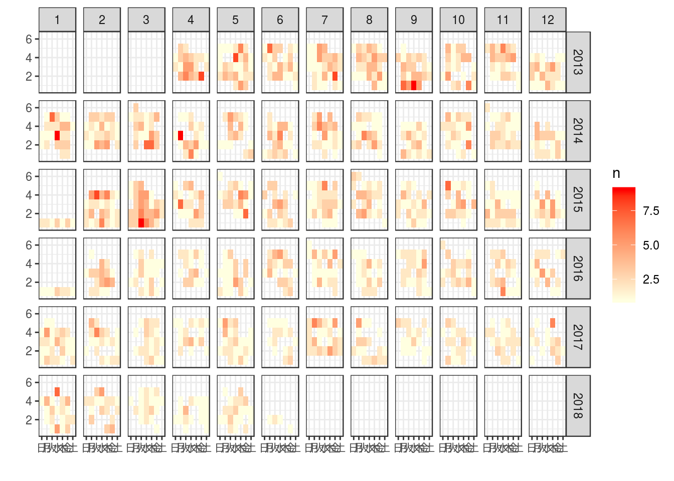
週次ヒートマップ
各月の第何曜日にピークがあるかを見る場合には月内週数計算に注意が必要です。月内週数を計算する関数がないため、週番号から月初日の週番号を差し引いて月内週数を求める必要があります。しかし、週番号は様々な定義があるため定義を理解していないと意図した結果にならない場合があります。
| 関数 | 処理概要 | 備考 |
|---|---|---|
lubridate::week |
1月1日を基準に7日単位で週番号を計算する | |
lubridate::isoweek |
ISO 8601にしたがって週番号を計算する | 月曜開始 |
lubridate::epiweek |
epidemiological week | 日曜開始 |
特にカレンダーをイメージした月内週数を得たい場合にはlubridate::isoweek関数を使用してください。ただし、 ISO 8601 の定義を理解しておく必要があります。
特に以下の点に注意してください。
- 週の始まりは月曜日
- 1月の最初の週は第52週や第53週になる場合がある(例:2016年1月)
- 12月の最終週は第1週になる場合がある(例:2013年12月30日)
月内週数は以下の計算で求められます。
月内週数を求めたい日(指定日)の週番号−月初日の週番号+1
R で計算する場合はlubridateパッケージを用います。ISO 8601で計算しますので、上記の注意事項を考慮して以下のようなコードになります。xは月内週数を計算したい日(指定日)です。
lubridate::isoweek(x) - lubridate::isoweek(lubridate::floor_date(x), "month") + offsetoffsetは以下のように条件により値が異なる点に注意してください。
| 条件 | offsetの値 | 備考 |
|---|---|---|
| 月初日の週番号が52週の場合 | 53 | |
| 月初日の週番号が53週の場合 | 54 | |
| 月初日の週番号が指定日の週番号より大きな場合 | 週番号 - 指定日の週番号 + 1 | |
| 上記以外 | 1 |
x %>%
  dplyr::filter(tracker == "Defect") %>%
  dplyr::select(date = open) %>%
  dplyr::mutate(date = lubridate::as_date(date)) %>%
# ヒートマップに項目に応じて年、月、週、日、曜日などを求める
  dplyr::mutate(year = lubridate::year(date), month = lubridate::month(date),
                week = lubridate::isoweek(date), day = lubridate::day(date),
                wday = lubridate::wday(date, label = TRUE, week_start = 1),
                tweek = lubridate::isoweek(lubridate::floor_date(date, "month"))) %>%
# ISO 8601に特有の処理
  dplyr::mutate(offset = ifelse(tweek == 53, 54, 1)) %>%
  dplyr::mutate(offset = ifelse(tweek == 52, 53, offset)) %>%
  dplyr::mutate(offset = ifelse(tweek > week, tweek - week + 1, offset)) %>%
# 例外処理
  dplyr::mutate(offset = ifelse(tweek == week, 1, offset)) %>%
# 月内の週数を計算する
  dplyr::mutate(mweek = week - tweek + offset) %>%
# 縦横軸でクロス集計する
  dplyr::count(mweek, wday) %>%
  ggplot2::ggplot(ggplot2::aes(x = mweek, y = wday, fill = n)) +
    ggplot2::geom_tile() +
    ggplot2::scale_fill_gradient(low = "lightyellow", high = "red") +
    ggplot2::labs(x = "", y = "曜日") +
    ggplot2::theme_bw() + ggplot2::scale_x_reverse() + ggplot2::coord_flip() +
    ggplot2::geom_text(ggplot2::aes(label = n))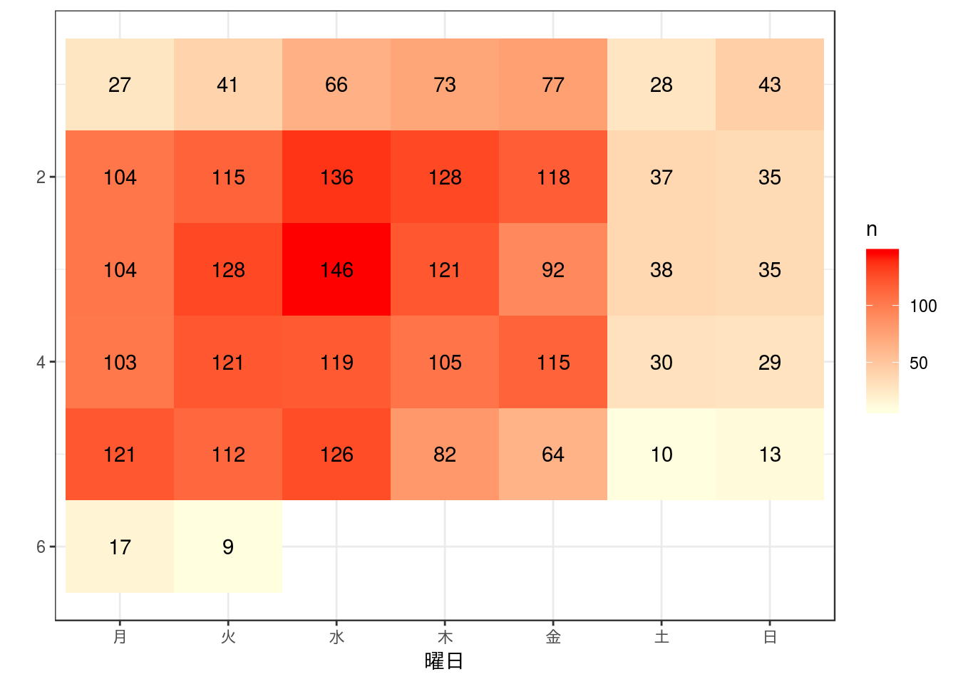
Tips
小計を加える
dplyrパッケージでクロス集計に小計を加える場合は以下のコードを参考にしてください。Sum列が行方向(各列)の小計、statusのNA行が列方向(各行)の小計になります。
row_sum <- x %>%
  dplyr::count(tracker, status) %>%
  tidyr::spread(key = tracker, value = n) %>%
  dplyr::mutate(Sum = ifelse(is.na(Defect), 0, Defect) +
                  ifelse(is.na(Patch), 0, Patch)) %>%
  dplyr::summarise_if(is.numeric, sum, na.rm = TRUE) %>%
  dplyr::mutate(status = NA) %>%
  dplyr::select(status, Defect, Patch, Sum)

x %>%
  dplyr::count(tracker, status) %>%
  tidyr::spread(key = tracker, value = n) %>%
  dplyr::mutate(Sum = ifelse(is.na(Defect), 0, Defect) +
                  ifelse(is.na(Patch), 0, Patch)) %>%
dplyr::bind_rows(row_sum)## # A tibble: 7 x 4
## status Defect Patch Sum
## <ord> <int> <int> <dbl>
## 1 New 504 176 680
## 2 Needs feedback 144 16 160
## 3 Confirmed 29 NA 29
## 4 Resolved 10 3 13
## 5 Closed 2174 760 2934
## 6 Reopened 7 3 10
## 7 <NA> 2868 958 3826